3. Business Cycles#

3.1. Overview#

In this lecture we review some empirical aspects of business cycles.

Business cycles are fluctuations in economic activity over time.

These include expansions (also called booms) and contractions (also called recessions).

For our study, we will use economic indicators from the World Bank and FRED.

In addition to the packages already installed by Anaconda, this lecture requires

!pip install wbgapi
!pip install pandas-datareader

Hide code cell output

Collecting wbgapi
  Downloading wbgapi-1.0.12-py3-none-any.whl.metadata (13 kB)
Requirement already satisfied: requests in /home/runner/miniconda3/envs/quantecon/lib/python3.13/site-packages (from wbgapi) (2.32.3)
Requirement already satisfied: PyYAML in /home/runner/miniconda3/envs/quantecon/lib/python3.13/site-packages (from wbgapi) (6.0.2)
Requirement already satisfied: tabulate in /home/runner/miniconda3/envs/quantecon/lib/python3.13/site-packages (from wbgapi) (0.9.0)
Requirement already satisfied: charset-normalizer<4,>=2 in /home/runner/miniconda3/envs/quantecon/lib/python3.13/site-packages (from requests->wbgapi) (3.3.2)
Requirement already satisfied: idna<4,>=2.5 in /home/runner/miniconda3/envs/quantecon/lib/python3.13/site-packages (from requests->wbgapi) (3.7)
Requirement already satisfied: urllib3<3,>=1.21.1 in /home/runner/miniconda3/envs/quantecon/lib/python3.13/site-packages (from requests->wbgapi) (2.3.0)
Requirement already satisfied: certifi>=2017.4.17 in /home/runner/miniconda3/envs/quantecon/lib/python3.13/site-packages (from requests->wbgapi) (2025.4.26)
Downloading wbgapi-1.0.12-py3-none-any.whl (36 kB)
Installing collected packages: wbgapi
Successfully installed wbgapi-1.0.12
Collecting pandas-datareader
  Downloading pandas_datareader-0.10.0-py3-none-any.whl.metadata (2.9 kB)
Requirement already satisfied: lxml in /home/runner/miniconda3/envs/quantecon/lib/python3.13/site-packages (from pandas-datareader) (5.3.0)
Requirement already satisfied: pandas>=0.23 in /home/runner/miniconda3/envs/quantecon/lib/python3.13/site-packages (from pandas-datareader) (2.2.3)
Requirement already satisfied: requests>=2.19.0 in /home/runner/miniconda3/envs/quantecon/lib/python3.13/site-packages (from pandas-datareader) (2.32.3)
Requirement already satisfied: numpy>=1.26.0 in /home/runner/miniconda3/envs/quantecon/lib/python3.13/site-packages (from pandas>=0.23->pandas-datareader) (2.1.3)
Requirement already satisfied: python-dateutil>=2.8.2 in /home/runner/miniconda3/envs/quantecon/lib/python3.13/site-packages (from pandas>=0.23->pandas-datareader) (2.9.0.post0)
Requirement already satisfied: pytz>=2020.1 in /home/runner/miniconda3/envs/quantecon/lib/python3.13/site-packages (from pandas>=0.23->pandas-datareader) (2024.1)
Requirement already satisfied: tzdata>=2022.7 in /home/runner/miniconda3/envs/quantecon/lib/python3.13/site-packages (from pandas>=0.23->pandas-datareader) (2025.2)
Requirement already satisfied: six>=1.5 in /home/runner/miniconda3/envs/quantecon/lib/python3.13/site-packages (from python-dateutil>=2.8.2->pandas>=0.23->pandas-datareader) (1.17.0)
Requirement already satisfied: charset-normalizer<4,>=2 in /home/runner/miniconda3/envs/quantecon/lib/python3.13/site-packages (from requests>=2.19.0->pandas-datareader) (3.3.2)
Requirement already satisfied: idna<4,>=2.5 in /home/runner/miniconda3/envs/quantecon/lib/python3.13/site-packages (from requests>=2.19.0->pandas-datareader) (3.7)
Requirement already satisfied: urllib3<3,>=1.21.1 in /home/runner/miniconda3/envs/quantecon/lib/python3.13/site-packages (from requests>=2.19.0->pandas-datareader) (2.3.0)
Requirement already satisfied: certifi>=2017.4.17 in /home/runner/miniconda3/envs/quantecon/lib/python3.13/site-packages (from requests>=2.19.0->pandas-datareader) (2025.4.26)
Downloading pandas_datareader-0.10.0-py3-none-any.whl (109 kB)
Installing collected packages: pandas-datareader
Successfully installed pandas-datareader-0.10.0

We use the following imports

import matplotlib.pyplot as plt
import pandas as pd
import datetime
import wbgapi as wb
import pandas_datareader.data as web

Here’s some minor code to help with colors in our plots.

Hide code cell source

# Set graphical parameters
cycler = plt.cycler(linestyle=['-', '-.', '--', ':'], 
        color=['#377eb8', '#ff7f00', '#4daf4a', '#ff334f'])
plt.rc('axes', prop_cycle=cycler)

3.2. Data acquisition#

We will use the World Bank’s data API wbgapi and pandas_datareader to retrieve data.

We can use wb.series.info with the argument q to query available data from the World Bank.

For example, let’s retrieve the GDP growth data ID to query GDP growth data.

wb.series.info(q='GDP growth')
id value
NY.GDP.MKTP.KD.ZGGDP growth (annual %)
1 elements

Now we use this series ID to obtain the data.

gdp_growth = wb.data.DataFrame('NY.GDP.MKTP.KD.ZG',
            ['USA', 'ARG', 'GBR', 'GRC', 'JPN'], 
            labels=True)
gdp_growth
Country YR1960 YR1961 YR1962 YR1963 YR1964 YR1965 YR1966 YR1967 YR1968 ... YR2015 YR2016 YR2017 YR2018 YR2019 YR2020 YR2021 YR2022 YR2023 YR2024
economy
JPN Japan NaN 12.043536 8.908973 8.473642 11.676708 5.819708 10.638562 11.082142 12.882468 ... 1.560627 0.753827 1.675332 0.643391 -0.402169 -4.168765 2.696574 0.941999 1.475035 0.083699
GRC Greece NaN 13.203839 0.364812 11.844867 9.409677 10.768011 6.494501 5.669486 7.203718 ... -0.228302 -0.031795 1.473125 2.064672 2.277181 -9.196231 8.654498 5.743649 2.332124 2.271736
GBR United Kingdom NaN 2.701314 1.098696 4.859545 5.594811 2.130333 1.567450 2.775738 5.472693 ... 2.222888 1.921710 2.656505 1.405190 1.624475 -10.296919 8.575951 4.839085 0.397082 1.100668
ARG Argentina NaN 5.427843 -0.852022 -5.308197 10.130298 10.569433 -0.659726 3.191997 4.822501 ... 2.731160 -2.080328 2.818503 -2.617396 -2.000861 -9.900485 10.441812 5.269880 -1.611002 -1.719105
USA United States NaN 2.565343 6.129637 4.357286 5.762747 6.498454 6.595342 2.742666 4.914509 ... 2.945550 1.819451 2.457622 2.966505 2.583825 -2.163029 6.055053 2.512375 2.887556 2.796190

5 rows × 66 columns

We can look at the series’ metadata to learn more about the series (click to expand).

wb.series.metadata.get('NY.GDP.MKTP.KD.ZG')

Hide code cell output

Series: NY.GDP.MKTP.KD.ZG

Field Value
Aggregationmethod Weighted average
Dataset WDI
Developmentrelevance This indicator is related to the national accounts, which are critical for understanding and managing a country's economy. They provide a framework for the analysis of economic performance. National accounts are the basis for estimating the Gross Domestic Product (GDP) and Gross National Income (GNI), which are the most widely used indicator of economic performance. They are essential for government policymakers, providing the data needed to design and assess fiscal and monetary policies; and are also used by businesses and investors to assess the economic climate and make investment decisions. NAS enable comparison between economies, which is crucial for international trade, investment decisions, and economic competitiveness. More specifically, this indicator is related to national accounts aggregates. Gross Domestic Product (GDP), Gross National Income (GNI), and other aggregates provide a snapshot of the size and health of an economy by measuring the total economic activity within a country. They can thus be used by policymakers to design and implement economic policies, as they reflect the overall economic performance and can indicate the need for intervention in certain areas. Aggregates also allow for comparisons between different economies, which can be useful for trade negotiations, investment decisions, and economic benchmarking. By examining aggregates over time, economists and analysts can identify trends, cycles, and potential areas of concern within an economy, and investors can use national accounts aggregates to assess the potential risks and returns of investing in a particular country. Overall, national accounts aggregates are fundamental tools for economic analysis, policy formulation, and decision-making at both the national and international levels.
IndicatorName GDP (annual % growth)
License_Type CC BY-4.0
License_URL https://creativecommons.org/licenses/by/4.0/
Limitationsandexceptions Each industry's contribution to growth in the economy's output is measured by growth in the industry's value added. In principle, value added in constant prices can be estimated by measuring the quantity of goods and services produced in a period, valuing them at an agreed set of base year prices, and subtracting the cost of intermediate inputs, also in constant prices. This double-deflation method requires detailed information on the structure of prices of inputs and outputs. In many industries, however, value added is extrapolated from the base year using single volume indexes of outputs or, less commonly, inputs. Particularly in the services industries, including most of government, value added in constant prices is often imputed from labor inputs, such as real wages or number of employees. In the absence of well defined measures of output, measuring the growth of services remains difficult. Moreover, technical progress can lead to improvements in production processes and in the quality of goods and services that, if not properly accounted for, can distort measures of value added and thus of growth. When inputs are used to estimate output, as for nonmarket services, unmeasured technical progress leads to underestimates of the volume of output. Similarly, unmeasured improvements in quality lead to underestimates of the value of output and value added. The result can be underestimates of growth and productivity improvement and overestimates of inflation. Informal economic activities pose a particular measurement problem, especially in developing countries, where much economic activity is unrecorded. A complete picture of the economy requires estimating household outputs produced for home use, sales in informal markets, barter exchanges, and illicit or deliberately unreported activities. The consistency and completeness of such estimates depend on the skill and methods of the compiling statisticians. Rebasing of national accounts can alter the measured growth rate of an economy and lead to breaks in series that affect the consistency of data over time. When countries rebase their national accounts, they update the weights assigned to various components to better reflect current patterns of production or uses of output. The new base year should represent normal operation of the economy - it should be a year without major shocks or distortions. Some developing countries have not rebased their national accounts for many years. Using an old base year can be misleading because implicit price and volume weights become progressively less relevant and useful. To obtain comparable series of constant price data for computing aggregates, the World Bank rescales GDP and value added by industrial origin to a common reference year. Because rescaling changes the implicit weights used in forming regional and income group aggregates, aggregate growth rates are not comparable with those from earlier editions with different base years. Rescaling may result in a discrepancy between the rescaled GDP and the sum of the rescaled components. To avoid distortions in the growth rates, the discrepancy is left unallocated. As a result, the weighted average of the growth rates of the components generally does not equal the GDP growth rate.
Longdefinition Gross domestic product is the total income earned through the production of goods and services in an economic territory during an accounting period. It can be measured in three different ways: using either the expenditure approach, the income approach, or the production approach. This indicator denotes the percentage change over each previous year of the constant price (base year 2015) series in United States dollars.
Periodicity Annual
Source Country official statistics, National Statistical Organizations and/or Central Banks; National Accounts data files, Organisation for Economic Co-operation and Development (OECD); Staff estimates, World Bank (WB)
StatisticalconceptandmethodologyMethodology: National accounts are compiled in accordance with international standards: System of National Accounts, 2008 or 1993 versions. Specific information on how countries compile their national accounts can be found on the IMF website: https://dsbb.imf.org/ Statistical concept(s): The conceptual elements of the SNA (System of National Accounts) measure what takes place in the economy, between which agents, and for what purpose. At the heart of the SNA is the production of goods and services. These may be used for consumption in the period to which the accounts relate or may be accumulated for use in a later period. In simple terms, the amount of value added generated by production represents GDP. The income corresponding to GDP is distributed to the various agents or groups of agents as income and it is the process of distributing and redistributing income that allows one agent to consume the goods and services produced by another agent or to acquire goods and services for later consumption. The way in which the SNA captures this pattern of economic flows is to identify the activities concerned by recognizing the institutional units in the economy and by specifying the structure of accounts capturing the transactions relevant to one stage or another of the process by which goods and services are produced and ultimately consumed.
Topic Economic Policy & Debt: National accounts: Growth rates
Unitofmeasure %

3.3. GDP growth rate#

First we look at GDP growth.

Let’s source our data from the World Bank and clean it.

# Use the series ID retrieved before
gdp_growth = wb.data.DataFrame('NY.GDP.MKTP.KD.ZG',
            ['USA', 'ARG', 'GBR', 'GRC', 'JPN'], 
            labels=True)
gdp_growth = gdp_growth.set_index('Country')
gdp_growth.columns = gdp_growth.columns.str.replace('YR', '').astype(int)

Here’s a first look at the data

gdp_growth
1960 1961 1962 1963 1964 1965 1966 1967 1968 1969 ... 2015 2016 2017 2018 2019 2020 2021 2022 2023 2024
Country
Japan NaN 12.043536 8.908973 8.473642 11.676708 5.819708 10.638562 11.082142 12.882468 12.477895 ... 1.560627 0.753827 1.675332 0.643391 -0.402169 -4.168765 2.696574 0.941999 1.475035 0.083699
Greece NaN 13.203839 0.364812 11.844867 9.409677 10.768011 6.494501 5.669486 7.203718 11.563668 ... -0.228302 -0.031795 1.473125 2.064672 2.277181 -9.196231 8.654498 5.743649 2.332124 2.271736
United Kingdom NaN 2.701314 1.098696 4.859545 5.594811 2.130333 1.567450 2.775738 5.472693 1.939138 ... 2.222888 1.921710 2.656505 1.405190 1.624475 -10.296919 8.575951 4.839085 0.397082 1.100668
Argentina NaN 5.427843 -0.852022 -5.308197 10.130298 10.569433 -0.659726 3.191997 4.822501 9.679526 ... 2.731160 -2.080328 2.818503 -2.617396 -2.000861 -9.900485 10.441812 5.269880 -1.611002 -1.719105
United States NaN 2.565343 6.129637 4.357286 5.762747 6.498454 6.595342 2.742666 4.914509 3.122477 ... 2.945550 1.819451 2.457622 2.966505 2.583825 -2.163029 6.055053 2.512375 2.887556 2.796190

5 rows × 65 columns

We write a function to generate plots for individual countries taking into account the recessions.

Hide code cell source

def plot_series(data, country, ylabel, 
                txt_pos, ax, g_params,
                b_params, t_params, ylim=15, baseline=0):
    """
    Plots a time series with recessions highlighted. 

    Parameters
    ----------
    data : pd.DataFrame
        Data to plot
    country : str
        Name of the country to plot
    ylabel : str
        Label of the y-axis
    txt_pos : float
        Position of the recession labels
    y_lim : float
        Limit of the y-axis
    ax : matplotlib.axes._subplots.AxesSubplot
        Axes to plot on
    g_params : dict
        Parameters for the line
    b_params : dict
        Parameters for the recession highlights
    t_params : dict
        Parameters for the recession labels
    baseline : float, optional
        Dashed baseline on the plot, by default 0
    
    Returns
    -------
    ax : matplotlib.axes.Axes
        Axes with the plot.
    """

    ax.plot(data.loc[country], label=country, **g_params)
    
    # Highlight recessions
    ax.axvspan(1973, 1975, **b_params)
    ax.axvspan(1990, 1992, **b_params)
    ax.axvspan(2007, 2009, **b_params)
    ax.axvspan(2019, 2021, **b_params)
    if ylim != None:
        ax.set_ylim([-ylim, ylim])
    else:
        ylim = ax.get_ylim()[1]
    ax.text(1974, ylim + ylim*txt_pos,
            'Oil Crisis\n(1974)', **t_params) 
    ax.text(1991, ylim + ylim*txt_pos,
            '1990s recession\n(1991)', **t_params) 
    ax.text(2008, ylim + ylim*txt_pos,
            'GFC\n(2008)', **t_params) 
    ax.text(2020, ylim + ylim*txt_pos,
            'Covid-19\n(2020)', **t_params)

    # Add a baseline for reference
    if baseline != None:
        ax.axhline(y=baseline, 
                   color='black', 
                   linestyle='--')
    ax.set_ylabel(ylabel)
    ax.legend()
    return ax

# Define graphical parameters 
g_params = {'alpha': 0.7}
b_params = {'color':'grey', 'alpha': 0.2}
t_params = {'color':'grey', 'fontsize': 9, 
            'va':'center', 'ha':'center'}

Let’s start with the United States.

fig, ax = plt.subplots()

country = 'United States'
ylabel = 'GDP growth rate (%)'
plot_series(gdp_growth, country, 
            ylabel, 0.1, ax, 
            g_params, b_params, t_params)
plt.show()
_images/fc83d0b76200f1b372d42f76ac1556555793de1c0c7bfda4512a6cfec9067d0b.png

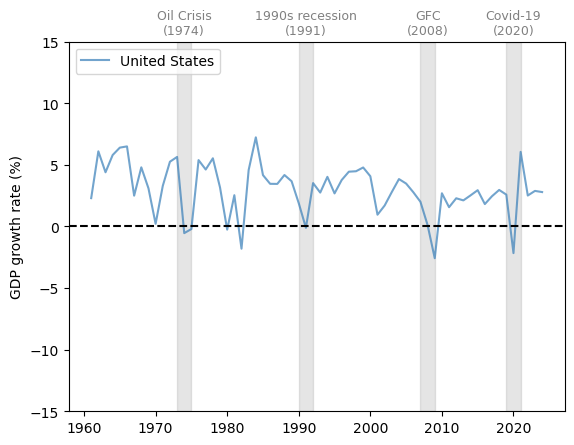
Fig. 3.1 United States (GDP growth rate %)#

GDP growth is positive on average and trending slightly downward over time.

We also see fluctuations over GDP growth over time, some of which are quite large.

Let’s look at a few more countries to get a basis for comparison.

The United Kingdom (UK) has a similar pattern to the US, with a slow decline in the growth rate and significant fluctuations.

Notice the very large dip during the Covid-19 pandemic.

fig, ax = plt.subplots()

country = 'United Kingdom'
plot_series(gdp_growth, country, 
            ylabel, 0.1, ax, 
            g_params, b_params, t_params)
plt.show()
_images/5b8fa0bd587c72245159d39d9d2c9026cd5e12907b57f843ac29484c0e839031.png

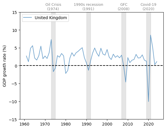
Fig. 3.2 United Kingdom (GDP growth rate %)#

Now let’s consider Japan, which experienced rapid growth in the 1960s and 1970s, followed by slowed expansion in the past two decades.

Major dips in the growth rate coincided with the Oil Crisis of the 1970s, the Global Financial Crisis (GFC) and the Covid-19 pandemic.

fig, ax = plt.subplots()

country = 'Japan'
plot_series(gdp_growth, country, 
            ylabel, 0.1, ax, 
            g_params, b_params, t_params)
plt.show()
_images/f57c34e5a3e665450ebb0bc20d3d63a176abc6209475d86c77888fdeafc87a37.png

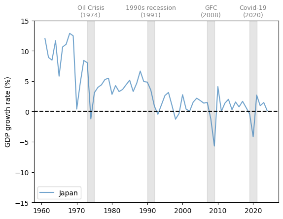
Fig. 3.3 Japan (GDP growth rate %)#

Now let’s study Greece.

fig, ax = plt.subplots()

country = 'Greece'
plot_series(gdp_growth, country, 
            ylabel, 0.1, ax, 
            g_params, b_params, t_params)
plt.show()
_images/884927279deb8cd47d77f7d313182024b225e13d35cf2569617f6069c1c3b060.png

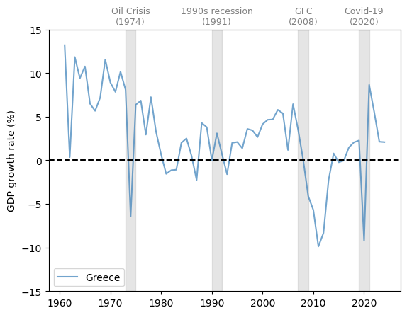
Fig. 3.4 Greece (GDP growth rate %)#

Greece experienced a very large drop in GDP growth around 2010-2011, during the peak of the Greek debt crisis.

Next let’s consider Argentina.

fig, ax = plt.subplots()

country = 'Argentina'
plot_series(gdp_growth, country, 
            ylabel, 0.1, ax, 
            g_params, b_params, t_params)
plt.show()
_images/c2d1a542871f52f8274ffe7063334d3fe7cfd94034a45d737816147ce575fd64.png

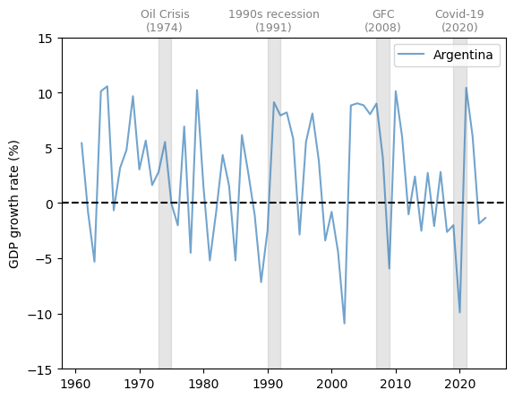
Fig. 3.5 Argentina (GDP growth rate %)#

Notice that Argentina has experienced far more volatile cycles than the economies examined above.

At the same time, Argentina’s growth rate did not fall during the two developed economy recessions in the 1970s and 1990s.

3.4. Unemployment#

Another important measure of business cycles is the unemployment rate.

We study unemployment using rate data from FRED spanning from 1929-1942 to 1948-2022, combined unemployment rate data over 1942-1948 estimated by the Census Bureau.

Hide code cell source

start_date = datetime.datetime(1929, 1, 1)
end_date = datetime.datetime(1942, 6, 1)

unrate_history = web.DataReader('M0892AUSM156SNBR', 
                    'fred', start_date,end_date)
unrate_history.rename(columns={'M0892AUSM156SNBR': 'UNRATE'}, 
                inplace=True)

start_date = datetime.datetime(1948, 1, 1)
end_date = datetime.datetime(2022, 12, 31)

unrate = web.DataReader('UNRATE', 'fred', 
                    start_date, end_date)

Let’s plot the unemployment rate in the US from 1929 to 2022 with recessions defined by the NBER.

Hide code cell source

# We use the census bureau's estimate for the unemployment rate 
# between 1942 and 1948
years = [datetime.datetime(year, 6, 1) for year in range(1942, 1948)]
unrate_census = [4.7, 1.9, 1.2, 1.9, 3.9, 3.9]

unrate_census = {'DATE': years, 'UNRATE': unrate_census}
unrate_census = pd.DataFrame(unrate_census)
unrate_census.set_index('DATE', inplace=True)

# Obtain the NBER-defined recession periods
start_date = datetime.datetime(1929, 1, 1)
end_date = datetime.datetime(2022, 12, 31)

nber = web.DataReader('USREC', 'fred', start_date, end_date)

fig, ax = plt.subplots()

ax.plot(unrate_history, **g_params, 
        color='#377eb8', 
        linestyle='-', linewidth=2)
ax.plot(unrate_census, **g_params, 
        color='black', linestyle='--', 
        label='Census estimates', linewidth=2)
ax.plot(unrate, **g_params, color='#377eb8', 
        linestyle='-', linewidth=2)

# Draw gray boxes according to NBER recession indicators
ax.fill_between(nber.index, 0, 1,
                where=nber['USREC']==1, 
                color='grey', edgecolor='none',
                alpha=0.3, 
                transform=ax.get_xaxis_transform(), 
                label='NBER recession indicators')
ax.set_ylim([0, ax.get_ylim()[1]])
ax.legend(loc='upper center', 
          bbox_to_anchor=(0.5, 1.1),
          ncol=3, fancybox=True, shadow=True)
ax.set_ylabel('unemployment rate (%)')

plt.show()
_images/6927dd8c658536c3f92c5deeacffa8285d169cfa902a4e032e73b8973a504205.png

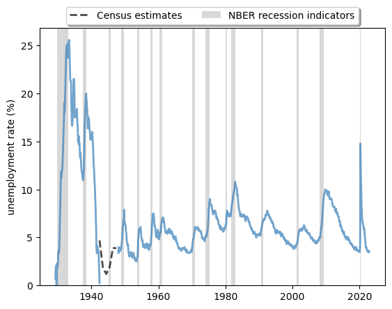
Fig. 3.6 Long-run unemployment rate, US (%)#

The plot shows that

  • expansions and contractions of the labor market have been highly correlated with recessions.

  • cycles are, in general, asymmetric: sharp rises in unemployment are followed by slow recoveries.

It also shows us how unique labor market conditions were in the US during the post-pandemic recovery.

The labor market recovered at an unprecedented rate after the shock in 2020-2021.

3.5. Synchronization#

In our previous discussion, we found that developed economies have had relatively synchronized periods of recession.

At the same time, this synchronization did not appear in Argentina until the 2000s.

Let’s examine this trend further.

With slight modifications, we can use our previous function to draw a plot that includes multiple countries.

Hide code cell source

def plot_comparison(data, countries, 
                        ylabel, txt_pos, y_lim, ax, 
                        g_params, b_params, t_params, 
                        baseline=0):
    """
    Plot multiple series on the same graph

    Parameters
    ----------
    data : pd.DataFrame
        Data to plot
    countries : list
        List of countries to plot
    ylabel : str
        Label of the y-axis
    txt_pos : float
        Position of the recession labels
    y_lim : float
        Limit of the y-axis
    ax : matplotlib.axes._subplots.AxesSubplot
        Axes to plot on
    g_params : dict
        Parameters for the lines
    b_params : dict
        Parameters for the recession highlights
    t_params : dict
        Parameters for the recession labels
    baseline : float, optional
        Dashed baseline on the plot, by default 0
    
    Returns
    -------
    ax : matplotlib.axes.Axes
        Axes with the plot.
    """
    
    # Allow the function to go through more than one series
    for country in countries:
        ax.plot(data.loc[country], label=country, **g_params)
    
    # Highlight recessions
    ax.axvspan(1973, 1975, **b_params)
    ax.axvspan(1990, 1992, **b_params)
    ax.axvspan(2007, 2009, **b_params)
    ax.axvspan(2019, 2021, **b_params)
    if y_lim != None:
        ax.set_ylim([-y_lim, y_lim])
    ylim = ax.get_ylim()[1]
    ax.text(1974, ylim + ylim*txt_pos, 
            'Oil Crisis\n(1974)', **t_params) 
    ax.text(1991, ylim + ylim*txt_pos, 
            '1990s recession\n(1991)', **t_params) 
    ax.text(2008, ylim + ylim*txt_pos, 
            'GFC\n(2008)', **t_params) 
    ax.text(2020, ylim + ylim*txt_pos, 
            'Covid-19\n(2020)', **t_params) 
    if baseline != None:
        ax.hlines(y=baseline, xmin=ax.get_xlim()[0], 
                  xmax=ax.get_xlim()[1], color='black', 
                  linestyle='--')
    ax.set_ylabel(ylabel)
    ax.legend()
    return ax

# Define graphical parameters 
g_params = {'alpha': 0.7}
b_params = {'color':'grey', 'alpha': 0.2}
t_params = {'color':'grey', 'fontsize': 9, 
            'va':'center', 'ha':'center'}

Here we compare the GDP growth rate of developed economies and developing economies.

Hide code cell source

# Obtain GDP growth rate for a list of countries
gdp_growth = wb.data.DataFrame('NY.GDP.MKTP.KD.ZG',
            ['CHN', 'USA', 'DEU', 'BRA', 'ARG', 'GBR', 'JPN', 'MEX'], 
            labels=True)
gdp_growth = gdp_growth.set_index('Country')
gdp_growth.columns = gdp_growth.columns.str.replace('YR', '').astype(int)

We use the United Kingdom, United States, Germany, and Japan as examples of developed economies.

Hide code cell source

fig, ax = plt.subplots()
countries = ['United Kingdom', 'United States', 'Germany', 'Japan']
ylabel = 'GDP growth rate (%)'
plot_comparison(gdp_growth.loc[countries, 1962:], 
                countries, ylabel,
                0.1, 20, ax, 
                g_params, b_params, t_params)
plt.show()
_images/1904ee737c233ae2447da3990ad48264e601f130429caf11a896ca91bab97927.png

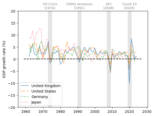
Fig. 3.7 Developed economies (GDP growth rate %)#

We choose Brazil, China, Argentina, and Mexico as representative developing economies.

Hide code cell source

fig, ax = plt.subplots()
countries = ['Brazil', 'China', 'Argentina', 'Mexico']
plot_comparison(gdp_growth.loc[countries, 1962:], 
                countries, ylabel, 
                0.1, 20, ax, 
                g_params, b_params, t_params)
plt.show()
_images/1b68f3b458d0a69beee64d1e36d14da3a5c22b98dcdc3a70c9a93062453d8e8f.png

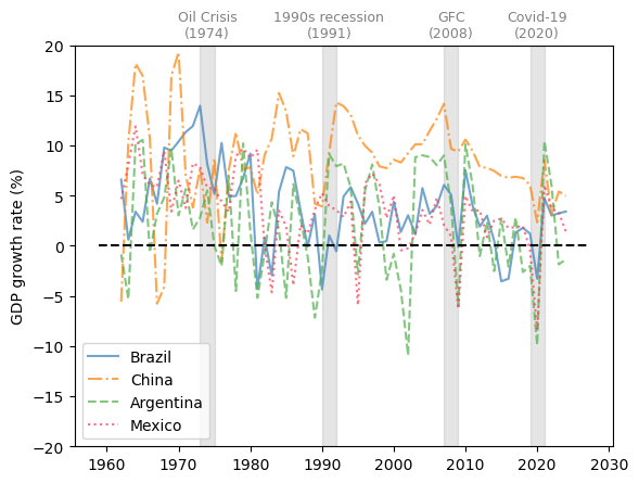
Fig. 3.8 Developing economies (GDP growth rate %)#

The comparison of GDP growth rates above suggests that business cycles are becoming more synchronized in 21st-century recessions.

However, emerging and less developed economies often experience more volatile changes throughout the economic cycles.

Despite the synchronization in GDP growth, the experience of individual countries during the recession often differs.

We use the unemployment rate and the recovery of labor market conditions as another example.

Here we compare the unemployment rate of the United States, the United Kingdom, Japan, and France.

Hide code cell source

unempl_rate = wb.data.DataFrame('SL.UEM.TOTL.NE.ZS',
    ['USA', 'FRA', 'GBR', 'JPN'], labels=True)
unempl_rate = unempl_rate.set_index('Country')
unempl_rate.columns = unempl_rate.columns.str.replace('YR', '').astype(int)

fig, ax = plt.subplots()

countries = ['United Kingdom', 'United States', 'Japan', 'France']
ylabel = 'unemployment rate (national estimate) (%)'
plot_comparison(unempl_rate, countries, 
                ylabel, 0.05, None, ax, g_params, 
                b_params, t_params, baseline=None)
plt.show()
_images/99e92d436ecb1ab3120dc1a350c8cf1cd13e63e807e0779177de915cf9774b9e.png

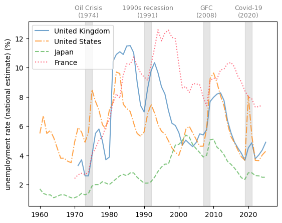
Fig. 3.9 Developed economies (unemployment rate %)#

We see that France, with its strong labor unions, typically experiences relatively slow labor market recoveries after negative shocks.

We also notice that Japan has a history of very low and stable unemployment rates.

3.6. Leading indicators and correlated factors#

Examining leading indicators and correlated factors helps policymakers to understand the causes and results of business cycles.

We will discuss potential leading indicators and correlated factors from three perspectives: consumption, production, and credit level.

3.6.1. Consumption#

Consumption depends on consumers’ confidence towards their income and the overall performance of the economy in the future.

One widely cited indicator for consumer confidence is the consumer sentiment index published by the University of Michigan.

Here we plot the University of Michigan Consumer Sentiment Index and year-on-year core consumer price index (CPI) change from 1978-2022 in the US.

Hide code cell source

start_date = datetime.datetime(1978, 1, 1)
end_date = datetime.datetime(2022, 12, 31)

# Limit the plot to a specific range
start_date_graph = datetime.datetime(1977, 1, 1)
end_date_graph = datetime.datetime(2023, 12, 31)

nber = web.DataReader('USREC', 'fred', start_date, end_date)
consumer_confidence = web.DataReader('UMCSENT', 'fred', 
                                start_date, end_date)

fig, ax = plt.subplots()
ax.plot(consumer_confidence, **g_params, 
        color='#377eb8', linestyle='-', 
        linewidth=2)
ax.fill_between(nber.index, 0, 1, 
            where=nber['USREC']==1, 
            color='grey', edgecolor='none',
            alpha=0.3, 
            transform=ax.get_xaxis_transform(), 
            label='NBER recession indicators')
ax.set_ylim([0, ax.get_ylim()[1]])
ax.set_ylabel('consumer sentiment index')

# Plot CPI on another y-axis
ax_t = ax.twinx()
inflation = web.DataReader('CPILFESL', 'fred', 
                start_date, end_date).pct_change(12)*100

# Add CPI on the legend without drawing the line again
ax_t.plot(2020, 0, **g_params, linestyle='-', 
          linewidth=2, label='consumer sentiment index')
ax_t.plot(inflation, **g_params, 
          color='#ff7f00', linestyle='--', 
          linewidth=2, label='CPI YoY change (%)')

ax_t.fill_between(nber.index, 0, 1,
                  where=nber['USREC']==1, 
                  color='grey', edgecolor='none',
                  alpha=0.3, 
                  transform=ax.get_xaxis_transform(), 
                  label='NBER recession indicators')
ax_t.set_ylim([0, ax_t.get_ylim()[1]])
ax_t.set_xlim([start_date_graph, end_date_graph])
ax_t.legend(loc='upper center',
            bbox_to_anchor=(0.5, 1.1),
            ncol=3, fontsize=9)
ax_t.set_ylabel('CPI YoY change (%)')
plt.show()
_images/7608f924c91e080329bb85f6291174bded60fe570317f9acb59b66436a8405f1.png

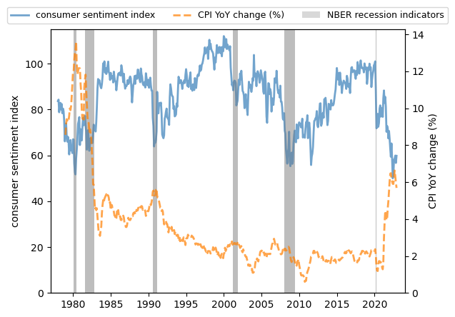
Fig. 3.10 Consumer sentiment index and YoY CPI change, US#

We see that

  • consumer sentiment often remains high during expansions and drops before recessions.

  • there is a clear negative correlation between consumer sentiment and the CPI.

When the price of consumer commodities rises, consumer confidence diminishes.

This trend is more significant during stagflation.

3.6.2. Production#

Real industrial output is highly correlated with recessions in the economy.

However, it is not a leading indicator, as the peak of contraction in production is delayed relative to consumer confidence and inflation.

We plot the real industrial output change from the previous year from 1919 to 2022 in the US to show this trend.

Hide code cell source

start_date = datetime.datetime(1919, 1, 1)
end_date = datetime.datetime(2022, 12, 31)

nber = web.DataReader('USREC', 'fred', 
                    start_date, end_date)
industrial_output = web.DataReader('INDPRO', 'fred', 
                    start_date, end_date).pct_change(12)*100

fig, ax = plt.subplots()
ax.plot(industrial_output, **g_params, 
        color='#377eb8', linestyle='-', 
        linewidth=2, label='Industrial production index')
ax.fill_between(nber.index, 0, 1,
                where=nber['USREC']==1, 
                color='grey', edgecolor='none',
                alpha=0.3, 
                transform=ax.get_xaxis_transform(), 
                label='NBER recession indicators')
ax.set_ylim([ax.get_ylim()[0], ax.get_ylim()[1]])
ax.set_ylabel('YoY real output change (%)')
plt.show()
_images/463a4c87959289ae227103e0db53e05e4450d0c616080c6683d9d4aceeded397.png

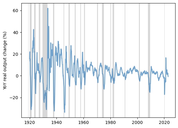
Fig. 3.11 YoY real output change, US (%)#

We observe the delayed contraction in the plot across recessions.

3.6.3. Credit level#

Credit contractions often occur during recessions, as lenders become more cautious and borrowers become more hesitant to take on additional debt.

This is due to factors such as a decrease in overall economic activity and gloomy expectations for the future.

One example is domestic credit to the private sector by banks in the UK.

The following graph shows the domestic credit to the private sector as a percentage of GDP by banks from 1970 to 2022 in the UK.

Hide code cell source

private_credit = wb.data.DataFrame('FS.AST.PRVT.GD.ZS', 
                ['GBR'], labels=True)
private_credit = private_credit.set_index('Country')
private_credit.columns = private_credit.columns.str.replace('YR', '').astype(int)

fig, ax = plt.subplots()

countries = 'United Kingdom'
ylabel = 'credit level (% of GDP)'
ax = plot_series(private_credit, countries, 
                 ylabel, 0.05, ax, g_params, b_params, 
                 t_params, ylim=None, baseline=None)
plt.show()
_images/e8266fbddcbd828f04f6380acf1887f094b97e01079c65b4a6bae3977494ad48.png

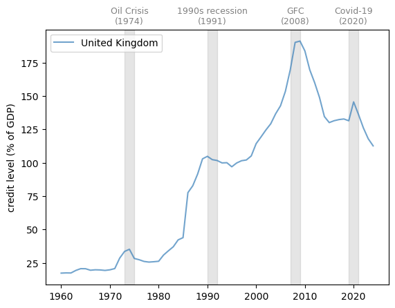
Fig. 3.12 Domestic credit to private sector by banks (% of GDP)#

Note that the credit rises during economic expansions and stagnates or even contracts after recessions.