5. Inflation During French Revolution#
5.1. Overview#
This lecture describes some of the monetary and fiscal features of the French Revolution (1789-1799) described by [Sargent and Velde, 1995].
To finance public expenditures and service its debts, the French government embarked on policy experiments.
The authors of these experiments had in mind theories about how government monetary and fiscal policies affected economic outcomes.
Some of those theories about monetary and fiscal policies still interest us today.
a tax-smoothing model like Robert Barro’s [Barro, 1979]
this normative (i.e., prescriptive model) advises a government to finance temporary war-time surges in expenditures mostly by issuing government debt, raising taxes by just enough to service the additional debt issued during the war; then, after the war, to roll over whatever debt the government had accumulated during the war; and to increase taxes after the war permanently by just enough to finance interest payments on that post-war government debt
unpleasant monetarist arithmetic like that described in this quantecon lecture Some Unpleasant Monetarist Arithmetic
mathematics involving compound interest governed French government debt dynamics in the decades preceding 1789; according to leading historians, that arithmetic set the stage for the French Revolution
a real bills theory of the effects of government open market operations in which the government backs new issues of paper money with government holdings of valuable real property or financial assets that holders of money can purchase from the government in exchange for their money.
The Revolutionaries learned about this theory from Adam Smith’s 1776 book The Wealth of Nations [Smith, 2010] and other contemporary sources
It shaped how the Revolutionaries issued a paper money called assignats from 1789 to 1791
a classical gold or silver standard
Napoleon Bonaparte became head of the French government in 1799. He used this theory to guide his monetary and fiscal policies
a classical inflation-tax theory of inflation in which Philip Cagan’s ([Cagan, 1956]) demand for money studied in this lecture A Monetarist Theory of Price Levels is a key component
This theory helps explain French price level and money supply data from 1794 to 1797
a legal restrictions or financial repression theory of the demand for real balances
The Twelve Members comprising the Committee of Public Safety who administered the Terror from June 1793 to July 1794 used this theory to shape their monetary policy
We use matplotlib to replicate several of the graphs with which [Sargent and Velde, 1995] portrayed outcomes of these experiments
5.2. Data Sources#
This lecture uses data from three spreadsheets assembled by [Sargent and Velde, 1995]:
import numpy as np
import pandas as pd
import matplotlib.pyplot as plt
plt.rcParams.update({'font.size': 12})

base_url = 'https://github.com/QuantEcon/lecture-python-intro/raw/'\
           + 'main/lectures/datasets/'

fig_3_url = f'{base_url}fig_3.xlsx'
dette_url = f'{base_url}dette.xlsx'
assignat_url = f'{base_url}assignat.xlsx'
5.3. Government Expenditures and Taxes Collected#
We’ll start by using matplotlib to construct several graphs that will provide important historical context.
These graphs are versions of ones that appear in [Sargent and Velde, 1995].
These graphs show that during the 18th century
government expenditures in France and Great Britain both surged during four big wars, and by comparable amounts
In Britain, tax revenues were approximately equal to government expenditures during peace times, but were substantially less than government expenditures during wars
In France, even in peace time, tax revenues were substantially less than government expenditures
# Read the data from Excel file
data2 = pd.read_excel(dette_url,
        sheet_name='Militspe', usecols='M:X',
        skiprows=7, nrows=102, header=None)

# French military spending, 1685-1789, in 1726 livres
data4 = pd.read_excel(dette_url,
        sheet_name='Militspe', usecols='D',
        skiprows=3, nrows=105, header=None).squeeze()

years = range(1685, 1790)

plt.figure()
plt.plot(years, data4, '*-', linewidth=0.8)

plt.plot(range(1689, 1791), data2.iloc[:, 4], linewidth=0.8)

plt.gca().spines['top'].set_visible(False)
plt.gca().spines['right'].set_visible(False)
plt.gca().tick_params(labelsize=12)
plt.xlim([1689, 1790])
plt.xlabel('*: France')
plt.ylabel('Millions of livres')
plt.ylim([0, 475])

plt.tight_layout()
plt.show()
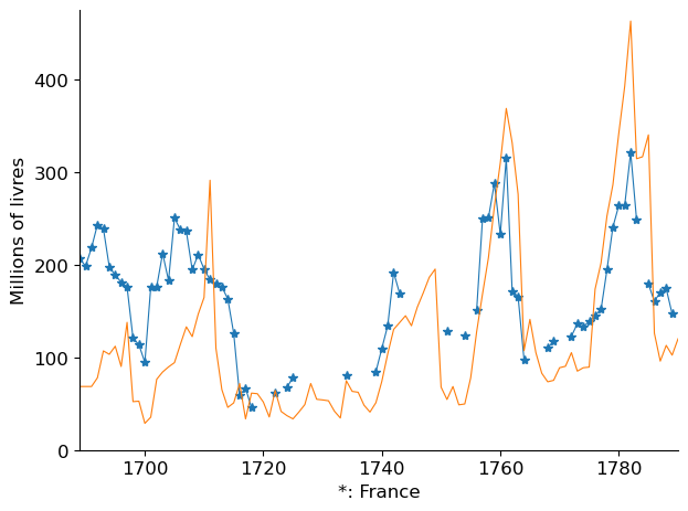
Fig. 5.1 Military Spending in Britain and France#
During the 18th century, Britain and France fought four large wars.
Britain won the first three wars and lost the fourth.
Each of those wars produced surges in both countries’ government expenditures that each country somehow had to finance.
Figure Fig. 5.1 shows surges in military expenditures in France (in blue) and Great Britain. during those four wars.
A remarkable aspect of figure Fig. 5.1 is that despite having a population less than half of France’s, Britain was able to finance military expenses of about the same amounts as France’s.
This testifies to Britain’s having created state institutions that could sustain high tax collections, government spending , and government borrowing. See [North and Weingast, 1989].
# Read the data from Excel file
data2 = pd.read_excel(dette_url, sheet_name='Militspe', usecols='M:X',
                      skiprows=7, nrows=102, header=None)

# Plot the data
plt.figure()
plt.plot(range(1689, 1791), data2.iloc[:, 5], linewidth=0.8)
plt.plot(range(1689, 1791), data2.iloc[:, 11], linewidth=0.8, color='red')
plt.plot(range(1689, 1791), data2.iloc[:, 9], linewidth=0.8, color='orange')
plt.plot(range(1689, 1791), data2.iloc[:, 8], 'o-',
         markerfacecolor='none', linewidth=0.8, color='purple')

# Customize the plot
plt.gca().spines['top'].set_visible(False)
plt.gca().spines['right'].set_visible(False)
plt.gca().tick_params(labelsize=12)
plt.xlim([1689, 1790])
plt.ylabel('millions of pounds', fontsize=12)

# Add text annotations
plt.text(1765, 1.5, 'civil', fontsize=10)
plt.text(1760, 4.2, 'civil plus debt service', fontsize=10)
plt.text(1708, 15.5, 'total govt spending', fontsize=10)
plt.text(1759, 7.3, 'revenues', fontsize=10)

plt.tight_layout()
plt.show()
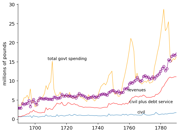
Fig. 5.2 Government Expenditures and Tax Revenues in Britain#
Figures Fig. 5.2 and Fig. 5.4 summarize British and French government fiscal policies during the century before the start of the French Revolution in 1789.
Before 1789, progressive forces in France admired how Britain had financed its government expenditures and wanted to redesign French fiscal arrangements to make them more like Britain’s.
Figure Fig. 5.2 shows government expenditures and how it was distributed among expenditures for
civil (non-military) activities
debt service, i.e., interest payments
military expenditures (the yellow line minus the red line)
Figure Fig. 5.2 also plots total government revenues from tax collections (the purple circled line)
Notice the surges in total government expenditures associated with surges in military expenditures in these four wars
Wars against France’s King Louis XIV early in the 18th century
The War of the Austrian Succession in the 1740s
The French and Indian War in the 1750’s and 1760s
The American War for Independence from 1775 to 1783
Figure Fig. 5.2 indicates that
during times of peace, government expenditures approximately equal taxes and debt service payments neither grow nor decline over time
during times of wars, government expenditures exceed tax revenues
the government finances the deficit of revenues relative to expenditures by issuing debt
after a war is over, the government’s tax revenues exceed its non-interest expenditures by just enough to service the debt that the government issued to finance earlier deficits
thus, after a war, the government does not raise taxes by enough to pay off its debt
instead, it just rolls over whatever debt it inherits, raising taxes by just enough to service the interest payments on that debt
Eighteenth-century British fiscal policy portrayed in Figure Fig. 5.2 thus looks very much like a text-book example of a tax-smoothing model like Robert Barro’s [Barro, 1979].
A striking feature of the graph is what we’ll label a law of gravity between tax collections and government expenditures.
levels of government expenditures and taxes attract each other
while they can temporarily differ – as they do during wars – they come back together when peace returns
Next we’ll plot data on debt service costs as fractions of government revenues in Great Britain and France during the 18th century.
# Read the data from the Excel file
data1 = pd.read_excel(dette_url, sheet_name='Debt',
            usecols='R:S', skiprows=5, nrows=99, header=None)
data1a = pd.read_excel(dette_url, sheet_name='Debt',
            usecols='P', skiprows=89, nrows=15, header=None)

# Plot the data
plt.figure()
plt.plot(range(1690, 1789), 100 * data1.iloc[:, 1], linewidth=0.8)

date = np.arange(1690, 1789)
index = (date < 1774) & (data1.iloc[:, 0] > 0)
plt.plot(date[index], 100 * data1[index].iloc[:, 0],
         '*:', color='r', linewidth=0.8)

# Plot the additional data
plt.plot(range(1774, 1789), 100 * data1a, '*:', color='orange')

# Note about the data
# The French data before 1720 don't match up with the published version
# Set the plot properties
plt.gca().spines['top'].set_visible(False)
plt.gca().spines['right'].set_visible(False)
plt.gca().set_facecolor('white')
plt.gca().set_xlim([1688, 1788])
plt.ylabel('% of Taxes')

plt.tight_layout()
plt.show()
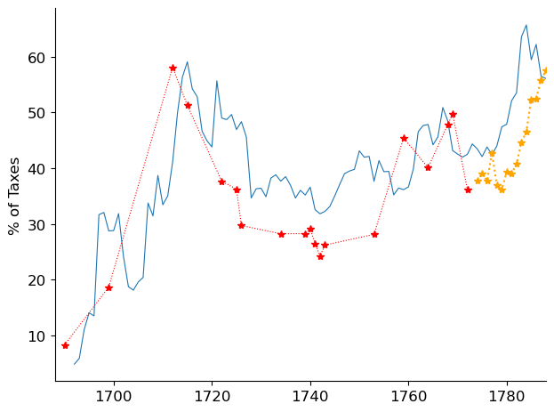
Fig. 5.3 Ratio of debt service to taxes, Britain and France#
Figure Fig. 5.3 shows that interest payments on government debt (i.e., so-called ‘‘debt service’’) were high fractions of government tax revenues in both Great Britain and France.
Fig. 5.2 showed us that in peace times Britain managed to balance its budget despite those large interest costs.
But as we’ll see in our next graph, on the eve of the French Revolution in 1788, the fiscal law of gravity that worked so well in Britain did not work very well in France.
# Read the data from the Excel file
data1 = pd.read_excel(fig_3_url, sheet_name='Sheet1',
          usecols='C:F', skiprows=5, nrows=30, header=None)

data1.replace(0, np.nan, inplace=True)
# Plot the data
plt.figure()

plt.plot(range(1759, 1789, 1), data1.iloc[:, 0], '-x', linewidth=0.8)
plt.plot(range(1759, 1789, 1), data1.iloc[:, 1], '--*', linewidth=0.8)
plt.plot(range(1759, 1789, 1), data1.iloc[:, 2],
         '-o', linewidth=0.8, markerfacecolor='none')
plt.plot(range(1759, 1789, 1), data1.iloc[:, 3], '-*', linewidth=0.8)

plt.text(1775, 610, 'total spending', fontsize=10)
plt.text(1773, 325, 'military', fontsize=10)
plt.text(1773, 220, 'civil plus debt service', fontsize=10)
plt.text(1773, 80, 'debt service', fontsize=10)
plt.text(1785, 500, 'revenues', fontsize=10)

plt.gca().spines['top'].set_visible(False)
plt.gca().spines['right'].set_visible(False)
plt.ylim([0, 700])
plt.ylabel('millions of livres')

plt.tight_layout()
plt.show()
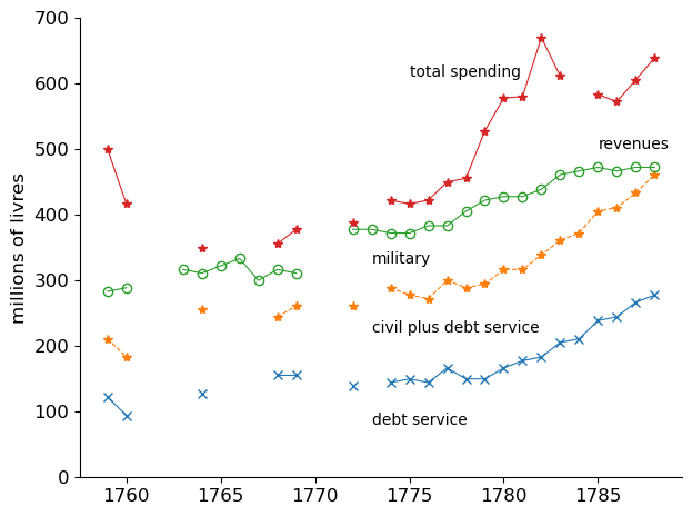
Fig. 5.4 Government Spending and Tax Revenues in France#
Fig. 5.4 shows that on the eve of the French Revolution in 1788, government expenditures exceeded tax revenues.
Especially during and after France’s expenditures to help the Americans in their War of Independence from Great Britain, growing government debt service (i.e., interest payments) contributed to this situation.
This was partly a consequence of the unfolding of the debt dynamics that underlies the Unpleasant Arithmetic discussed in this quantecon lecture Some Unpleasant Monetarist Arithmetic.
[Sargent and Velde, 1995] describe how the Ancient Regime that until 1788 had governed France had stable institutional features that made it difficult for the government to balance its budget.
Powerful contending interests had prevented the government from closing the gap between its total expenditures and its tax revenues by either
raising taxes, or
lowering government’s non-debt service (i.e., non-interest) expenditures, or
lowering debt service (i.e., interest) costs by rescheduling, i.e., defaulting on some debts
Precedents and prevailing French arrangements had empowered three constituencies to block adjustments to components of the government budget constraint that they cared especially about
tax payers
beneficiaries of government expenditures
government creditors (i.e., owners of government bonds)
When the French government had confronted a similar situation around 1720 after King Louis XIV’s Wars had left it with a debt crisis, it had sacrificed the interests of government creditors, i.e., by defaulting on enough of its debt to bring interest payments down enough to balance the budget.
Somehow, in 1789, creditors of the French government were more powerful than they had been in 1720.
Therefore, King Louis XVI convened the Estates General together to ask them to redesign the French constitution in a way that would lower government expenditures or increase taxes, thereby allowing him to balance the budget while also honoring his promises to creditors of the French government.
The King called the Estates General together in an effort to promote the reforms that would bring sustained budget balance.
[Sargent and Velde, 1995] describe how the French Revolutionaries set out to accomplish that.
5.4. Nationalization, Privatization, Debt Reduction#
In 1789, the Revolutionaries quickly reorganized the Estates General into a National Assembly.
A first piece of business was to address the fiscal crisis, the situation that had motivated the King to convene the Estates General.
The Revolutionaries were not socialists or communists.
To the contrary, they respected private property and knew state-of-the-art economics.
They knew that to honor government debts, they would have to raise new revenues or reduce expenditures.
A coincidence was that the Catholic Church owned vast income-producing properties.
Indeed, the capitalized value of those income streams put estimates of the value of church lands at about the same amount as the entire French government debt.
This coincidence fostered a three step plan for servicing the French government debt
nationalize the church lands – i.e., sequester or confiscate them without paying for them
sell the church lands
use the proceeds from those sales to service or even retire French government debt
The monetary theory underlying this plan had been set out by Adam Smith in his analysis of what he called real bills in his 1776 book The Wealth of Nations [Smith, 2010], which many of the revolutionaries had read.
Adam Smith defined a real bill as a paper money note that is backed by a claim on a real asset like productive capital or inventories.
The National Assembly put together an ingenious institutional arrangement to implement this plan.
In response to a motion by Catholic Bishop Talleyrand (an atheist), the National Assembly confiscated and nationalized Church lands.
The National Assembly intended to use earnings from Church lands to service its national debt.
To do this, it began to implement a ‘‘privatization plan’’ that would let it service its debt while not raising taxes.
Their plan involved issuing paper notes called ‘‘assignats’’ that entitled bearers to use them to purchase state lands.
These paper notes would be ‘‘as good as silver coins’’ in the sense that both were acceptable means of payment in exchange for those (formerly) church lands.
Finance Minister Necker and the Constituents of the National Assembly thus planned to solve the privatization problem and the debt problem simultaneously by creating a new currency.
They devised a scheme to raise revenues by auctioning the confiscated lands, thereby withdrawing paper notes issued on the security of the lands sold by the government.
This ‘‘tax-backed money’’ scheme propelled the National Assembly into the domains of then modern monetary theories.
Records of debates show how members of the Assembly marshaled theory and evidence to assess the likely effects of their innovation.
Members of the National Assembly quoted David Hume and Adam Smith
They cited John Law’s System of 1720 and the American experiences with paper money fifteen years earlier as examples of how paper money schemes can go awry
Knowing pitfalls, they set out to avoid them
They succeeded for two or three years.
But after that, France entered a big War that disrupted the plan in ways that completely altered the character of France’s paper money. [Sargent and Velde, 1995] describe what happened.
5.5. Remaking the tax code and tax administration#
In 1789 the French Revolutionaries formed a National Assembly and set out to remake French fiscal policy.
They wanted to honor government debts – interests of French government creditors were well represented in the National Assembly.
But they set out to remake the French tax code and the administrative machinery for collecting taxes.
they abolished many taxes
they abolished the Ancient Regime’s scheme for tax farming
tax farming meant that the government had privatized tax collection by hiring private citizens – so-called tax farmers to collect taxes, while retaining a fraction of them as payment for their services
the great chemist Lavoisier was also a tax farmer, one of the reasons that the Committee for Public Safety sent him to the guillotine in 1794
As a consequence of these tax reforms, government tax revenues declined
The next figure shows this
# Read data from Excel file
data5 = pd.read_excel(dette_url, sheet_name='Debt', usecols='K',
                    skiprows=41, nrows=120, header=None)

# Plot the data
plt.figure()
plt.plot(range(1726, 1846), data5.iloc[:, 0], linewidth=0.8)

plt.gca().spines['top'].set_visible(False)
plt.gca().spines['right'].set_visible(False)
plt.gca().set_facecolor('white')
plt.gca().tick_params(labelsize=12)
plt.xlim([1726, 1845])
plt.ylabel('1726 = 1', fontsize=12)

plt.tight_layout()
plt.show()
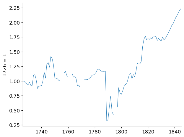
Fig. 5.5 Index of real per capita revenues, France#
According to Fig. 5.5, tax revenues per capita did not rise to their pre 1789 levels until after 1815, when Napoleon Bonaparte was exiled to St Helena and King Louis XVIII was restored to the French Crown.
from 1799 to 1814, Napoleon Bonaparte had other sources of revenues – booty and reparations from provinces and nations that he defeated in war
from 1789 to 1799, the French Revolutionaries turned to another source to raise resources to pay for government purchases of goods and services and to service French government debt.
And as the next figure shows, government expenditures exceeded tax revenues by substantial amounts during the period from 1789 to 1799.
# Read data from Excel file
data11 = pd.read_excel(assignat_url, sheet_name='Budgets',
        usecols='J:K', skiprows=22, nrows=52, header=None)

# Prepare the x-axis data
x_data = np.concatenate([
    np.arange(1791, 1794 + 8/12, 1/12),
    np.arange(1794 + 9/12, 1795 + 3/12, 1/12)
])

# Remove NaN values from the data
data11_clean = data11.dropna()

# Plot the data
plt.figure()
h = plt.plot(x_data, data11_clean.values[:, 0], linewidth=0.8)
h = plt.plot(x_data, data11_clean.values[:, 1], '--', linewidth=0.8)

# Set plot properties
plt.gca().spines['top'].set_visible(False)
plt.gca().spines['right'].set_visible(False)
plt.gca().set_facecolor('white')
plt.gca().tick_params(axis='both', which='major', labelsize=12)
plt.xlim([1791, 1795 + 3/12])
plt.xticks(np.arange(1791, 1796))
plt.yticks(np.arange(0, 201, 20))

# Set the y-axis label
plt.ylabel('millions of livres', fontsize=12)

plt.tight_layout()
plt.show()
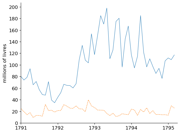
Fig. 5.6 Spending (blue) and Revenues (orange), (real values)#
To cover the discrepancies between government expenditures and tax revenues revealed in Fig. 5.6, the French revolutionaries printed paper money and spent it.
The next figure shows that by printing money, they were able to finance substantial purchases of goods and services, including military goods and soldiers’ pay.
# Read data from Excel file
data12 = pd.read_excel(assignat_url, sheet_name='seignor',
         usecols='F', skiprows=6, nrows=75, header=None).squeeze()

# Create a figure and plot the data
plt.figure()
plt.plot(pd.date_range(start='1790', periods=len(data12), freq='ME'),
         data12, linewidth=0.8)

plt.gca().spines['top'].set_visible(False)
plt.gca().spines['right'].set_visible(False)

plt.axhline(y=472.42/12, color='r', linestyle=':')
plt.xticks(ticks=pd.date_range(start='1790',
           end='1796', freq='YS'), labels=range(1790, 1797))
plt.xlim(pd.Timestamp('1791'),
         pd.Timestamp('1796-02') + pd.DateOffset(months=2))
plt.ylabel('millions of livres', fontsize=12)
plt.text(pd.Timestamp('1793-11'), 39.5, 'revenues in 1788',
         verticalalignment='top', fontsize=12)

plt.tight_layout()
plt.show()
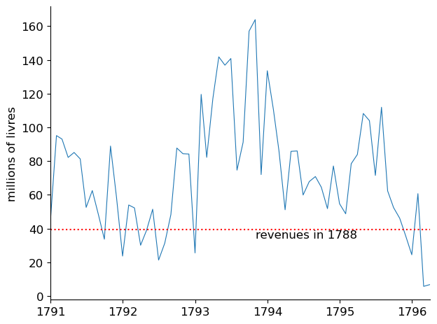
Fig. 5.7 Revenues raised by printing paper money notes#
Fig. 5.7 compares the revenues raised by printing money from 1789 to 1796 with tax revenues that the Ancient Regime had raised in 1788.
Measured in goods, revenues raised at time \(t\) by printing new money equal
where
\(M_t\) is the stock of paper money at time \(t\) measured in livres
\(p_t\) is the price level at time \(t\) measured in units of goods per livre at time \(t\)
\(M_{t+1} - M_t\) is the amount of new money printed at time \(t\)
Notice the 1793-1794 surge in revenues raised by printing money.
This reflects extraordinary measures that the Committee for Public Safety adopted to force citizens to accept paper money, or else.
Also note the abrupt fall off in revenues raised by 1797 and the absence of further observations after 1797.
This reflects the end of using the printing press to raise revenues.
What French paper money entitled its holders to changed over time in interesting ways.
These led to outcomes that vary over time and that illustrate the playing out in practice of theories that guided the Revolutionaries’ monetary policy decisions.
The next figure shows the price level in France during the time that the Revolutionaries used paper money to finance parts of their expenditures.
Note that we use a log scale because the price level rose so much.
# Read the data from Excel file
data7 = pd.read_excel(assignat_url, sheet_name='Data',
          usecols='P:Q', skiprows=4, nrows=80, header=None)
data7a = pd.read_excel(assignat_url, sheet_name='Data',
          usecols='L', skiprows=4, nrows=80, header=None)
# Create the figure and plot
plt.figure()
x = np.arange(1789 + 10/12, 1796 + 5/12, 1/12)
h, = plt.plot(x, 1. / data7.iloc[:, 0], linestyle='--')
h, = plt.plot(x, 1. / data7.iloc[:, 1], color='r')

# Set properties of the plot
plt.gca().tick_params(labelsize=12)
plt.yscale('log')
plt.xlim([1789 + 10/12, 1796 + 5/12])
plt.gca().spines['top'].set_visible(False)
plt.gca().spines['right'].set_visible(False)

# Add vertical lines
plt.axvline(x=1793 + 6.5/12, linestyle='-', linewidth=0.8, color='orange')
plt.axvline(x=1794 + 6.5/12, linestyle='-', linewidth=0.8, color='purple')

# Add text
plt.text(1793.75, 120, 'Terror', fontsize=12)
plt.text(1795, 2.8, 'price level', fontsize=12)
plt.text(1794.9, 40, 'gold', fontsize=12)


plt.tight_layout()
plt.show()
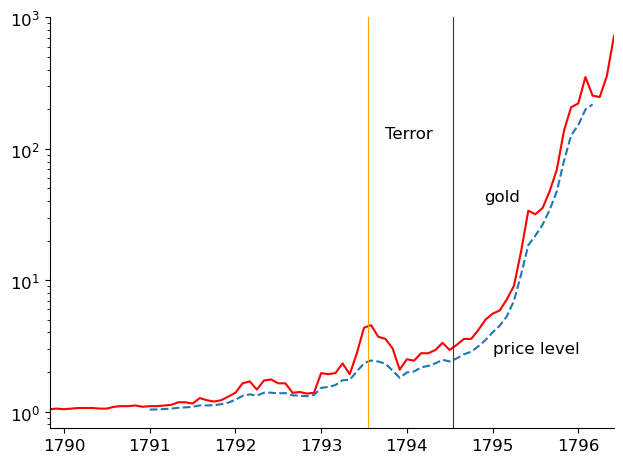
Fig. 5.8 Price Level and Price of Gold (log scale)#
We have partitioned Fig. 5.8 that shows the log of the price level and Fig. 5.9 below that plots real balances \(\frac{M_t}{p_t}\) into three periods that correspond to different monetary experiments or regimes.
The first period ends in the late summer of 1793, and is characterized by growing real balances and moderate inflation.
The second period begins and ends with the Terror. It is marked by high real balances, around 2,500 million, and roughly stable prices. The fall of Robespierre in late July 1794 begins the third of our episodes, in which real balances decline and prices rise rapidly.
We interpret these three episodes in terms of distinct theories
a backing or real bills theory (the classic text for this theory is Adam Smith [Smith, 2010])
a legal restrictions theory ( [Keynes, 1940], [Bryant and Wallace, 1984] )
a classical hyperinflation theory ([Cagan, 1956])
Note
According to the empirical definition of hyperinflation adopted by [Cagan, 1956], beginning in the month that inflation exceeds 50 percent per month and ending in the month before inflation drops below 50 percent per month for at least a year, the assignat experienced a hyperinflation from May to December 1795.
We view these theories not as competitors but as alternative collections of ‘‘if-then’’ statements about government note issues, each of which finds its conditions more nearly met in one of these episodes than in the other two.
# Read the data from Excel file
data7 = pd.read_excel(assignat_url, sheet_name='Data',
        usecols='P:Q', skiprows=4, nrows=80, header=None)
data7a = pd.read_excel(assignat_url, sheet_name='Data',
        usecols='L', skiprows=4, nrows=80, header=None)

# Create the figure and plot
plt.figure()
h = plt.plot(pd.date_range(start='1789-11-01', periods=len(data7), freq='ME'),
            (data7a.values * [1, 1]) * data7.values, linewidth=1.)
plt.setp(h[1], linestyle='--', color='red')

plt.vlines([pd.Timestamp('1793-07-15'), pd.Timestamp('1793-07-15')],
           0, 3000, linewidth=0.8, color='orange')
plt.vlines([pd.Timestamp('1794-07-15'), pd.Timestamp('1794-07-15')],
           0, 3000, linewidth=0.8, color='purple')

plt.ylim([0, 3000])

# Set properties of the plot
plt.gca().spines['top'].set_visible(False)
plt.gca().spines['right'].set_visible(False)
plt.gca().set_facecolor('white')
plt.gca().tick_params(labelsize=12)
plt.xlim(pd.Timestamp('1789-11-01'), pd.Timestamp('1796-06-01'))
plt.ylabel('millions of livres', fontsize=12)

# Add text annotations
plt.text(pd.Timestamp('1793-09-01'), 200, 'Terror', fontsize=12)
plt.text(pd.Timestamp('1791-05-01'), 750, 'gold value', fontsize=12)
plt.text(pd.Timestamp('1794-10-01'), 2500, 'real value', fontsize=12)


plt.tight_layout()
plt.show()
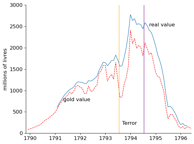
Fig. 5.9 Real balances of assignats (in gold and goods)#
The three clouds of points in Figure Fig. 5.10 depict different real balance-inflation relationships.
Only the cloud for the third period has the inverse relationship familiar to us now from twentieth-century hyperinflations.
subperiod 1: (”real bills period): January 1791 to July 1793
subperiod 2: (“terror”): August 1793 - July 1794
subperiod 3: (“classic Cagan hyperinflation”): August 1794 - March 1796
def fit(x, y):

    b = np.cov(x, y)[0, 1] / np.var(x)
    a = y.mean() - b * x.mean()

    return a, b
# Load data
caron = np.load('datasets/caron.npy')
nom_balances = np.load('datasets/nom_balances.npy')

infl = np.concatenate(([np.nan],
      -np.log(caron[1:63, 1] / caron[0:62, 1])))
bal = nom_balances[14:77, 1] * caron[:, 1] / 1000
# Regress y on x for three periods
a1, b1 = fit(bal[1:31], infl[1:31])
a2, b2 = fit(bal[31:44], infl[31:44])
a3, b3 = fit(bal[44:63], infl[44:63])

# Regress x on y for three periods
a1_rev, b1_rev = fit(infl[1:31], bal[1:31])
a2_rev, b2_rev = fit(infl[31:44], bal[31:44])
a3_rev, b3_rev = fit(infl[44:63], bal[44:63])
plt.figure()
plt.gca().spines['top'].set_visible(False)
plt.gca().spines['right'].set_visible(False)

# First subsample
plt.plot(bal[1:31], infl[1:31], 'o', markerfacecolor='none',
         color='blue', label='real bills period')

# Second subsample
plt.plot(bal[31:44], infl[31:44], '+', color='red', label='terror')

# Third subsample
plt.plot(bal[44:63], infl[44:63], '*',
        color='orange', label='classic Cagan hyperinflation')

plt.xlabel('real balances')
plt.ylabel('inflation')
plt.legend()

plt.tight_layout()
plt.show()
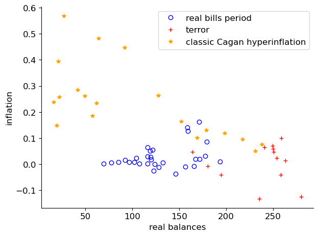
Fig. 5.10 Inflation and Real Balances#
The three clouds of points in Fig. 5.10 evidently depict different real balance-inflation relationships.
Only the cloud for the third period has the inverse relationship familiar to us now from twentieth-century hyperinflations.
To bring this out, we’ll use linear regressions to draw straight lines that compress the inflation-real balance relationship for our three sub-periods.
Before we do that, we’ll drop some of the early observations during the terror period to obtain the following graph.
# Regress y on x for three periods
a1, b1 = fit(bal[1:31], infl[1:31])
a2, b2 = fit(bal[31:44], infl[31:44])
a3, b3 = fit(bal[44:63], infl[44:63])

# Regress x on y for three periods
a1_rev, b1_rev = fit(infl[1:31], bal[1:31])
a2_rev, b2_rev = fit(infl[31:44], bal[31:44])
a3_rev, b3_rev = fit(infl[44:63], bal[44:63])
plt.figure()
plt.gca().spines['top'].set_visible(False)
plt.gca().spines['right'].set_visible(False)

# First subsample
plt.plot(bal[1:31], infl[1:31], 'o', markerfacecolor='none', color='blue', label='real bills period')

# Second subsample
plt.plot(bal[34:44], infl[34:44], '+', color='red', label='terror')

# Third subsample
plt.plot(bal[44:63], infl[44:63], '*', color='orange', label='classic Cagan hyperinflation')

plt.xlabel('real balances')
plt.ylabel('inflation')
plt.legend()

plt.tight_layout()
plt.show()
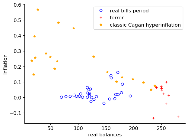
Fig. 5.11 Inflation and Real Balances#
Now let’s regress inflation on real balances during the real bills period and plot the regression line.
plt.figure()
plt.gca().spines['top'].set_visible(False)
plt.gca().spines['right'].set_visible(False)

# First subsample
plt.plot(bal[1:31], infl[1:31], 'o', markerfacecolor='none',
        color='blue', label='real bills period')
plt.plot(bal[1:31], a1 + bal[1:31] * b1, color='blue')

# Second subsample
plt.plot(bal[31:44], infl[31:44], '+', color='red', label='terror')

# Third subsample
plt.plot(bal[44:63], infl[44:63], '*',
        color='orange', label='classic Cagan hyperinflation')

plt.xlabel('real balances')
plt.ylabel('inflation')
plt.legend()

plt.tight_layout()
plt.show()
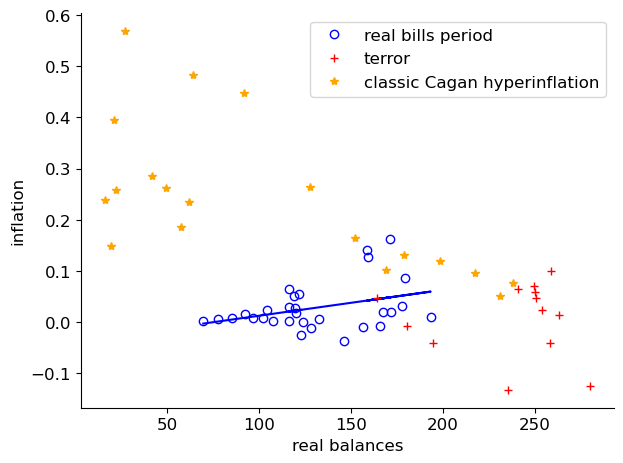
Fig. 5.12 Inflation and Real Balances#
The regression line in Fig. 5.12 shows that large increases in real balances of assignats (paper money) were accompanied by only modest rises in the price level, an outcome in line with the real bills theory.
During this period, assignats were claims on church lands.
But towards the end of this period, the price level started to rise and real balances to fall as the government continued to print money but stopped selling church land.
To get people to hold that paper money, the government forced people to hold it by using legal restrictions.
Now let’s regress real balances on inflation during the terror and plot the regression line.
plt.figure()
plt.gca().spines['top'].set_visible(False)
plt.gca().spines['right'].set_visible(False)

# First subsample
plt.plot(bal[1:31], infl[1:31], 'o', markerfacecolor='none',
        color='blue', label='real bills period')

# Second subsample
plt.plot(bal[31:44], infl[31:44], '+', color='red', label='terror')
plt.plot(a2_rev + b2_rev * infl[31:44], infl[31:44], color='red')

# Third subsample
plt.plot(bal[44:63], infl[44:63], '*',
        color='orange', label='classic Cagan hyperinflation')

plt.xlabel('real balances')
plt.ylabel('inflation')
plt.legend()

plt.tight_layout()
plt.show()
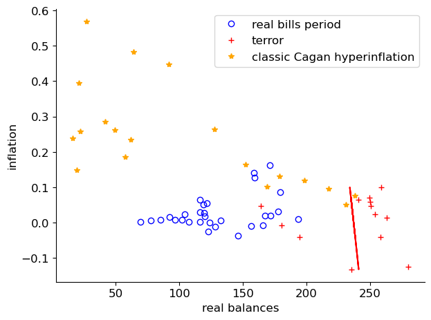
Fig. 5.13 Inflation and Real Balances#
The regression line in Fig. 5.13 shows that large increases in real balances of assignats (paper money) were accompanied by little upward price level pressure, even some declines in prices.
This reflects how well legal restrictions – financial repression – was working during the period of the Terror.
But the Terror ended in July 1794.
That unleashed a big inflation as people tried to find other ways to transact and store values.
The following two graphs are for the classical hyperinflation period.
One regresses inflation on real balances, the other regresses real balances on inflation.
Both show a pronounced inverse relationship that is the hallmark of the hyperinflations studied by Cagan [Cagan, 1956].
plt.figure()
plt.gca().spines['top'].set_visible(False)
plt.gca().spines['right'].set_visible(False)

# First subsample
plt.plot(bal[1:31], infl[1:31], 'o', markerfacecolor='none',
        color='blue', label='real bills period')

# Second subsample
plt.plot(bal[31:44], infl[31:44], '+', color='red', label='terror')

# Third subsample
plt.plot(bal[44:63], infl[44:63], '*',
    color='orange', label='classic Cagan hyperinflation')
plt.plot(bal[44:63], a3 + bal[44:63] * b3, color='orange')

plt.xlabel('real balances')
plt.ylabel('inflation')
plt.legend()

plt.tight_layout()
plt.show()
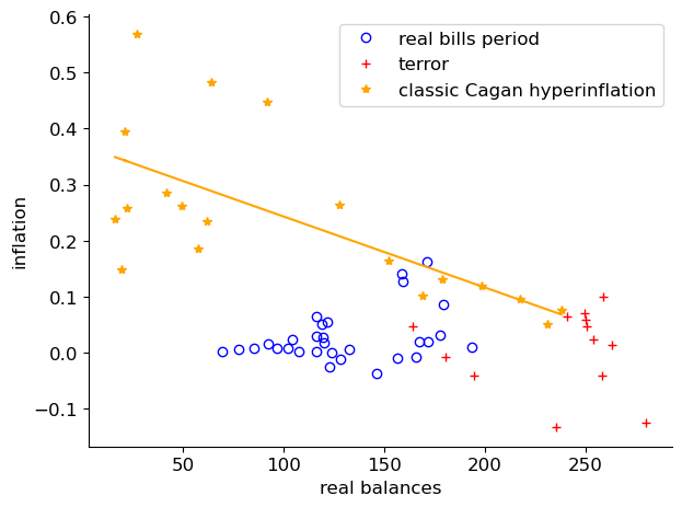
Fig. 5.14 Inflation and Real Balances#
Fig. 5.14 shows the results of regressing inflation on real balances during the period of the hyperinflation.
plt.figure()
plt.gca().spines['top'].set_visible(False)
plt.gca().spines['right'].set_visible(False)

# First subsample
plt.plot(bal[1:31], infl[1:31], 'o',
    markerfacecolor='none', color='blue', label='real bills period')

# Second subsample
plt.plot(bal[31:44], infl[31:44], '+', color='red', label='terror')

# Third subsample
plt.plot(bal[44:63], infl[44:63], '*',
        color='orange', label='classic Cagan hyperinflation')
plt.plot(a3_rev + b3_rev * infl[44:63], infl[44:63], color='orange')

plt.xlabel('real balances')
plt.ylabel('inflation')
plt.legend()

plt.tight_layout()
plt.show()
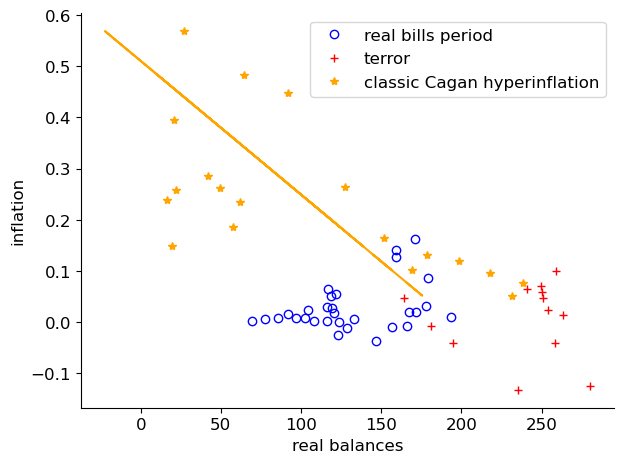
Fig. 5.15 Inflation and Real Balances#
Fig. 5.14 shows the results of regressing real money balances on inflation during the period of the hyperinflation.
5.6. Hyperinflation Ends#
[Sargent and Velde, 1995] tell how in 1797 the Revolutionary government abruptly ended the inflation by
repudiating 2/3 of the national debt, and thereby
eliminating the net-of-interest government deficit
no longer printing money, but instead
using gold and silver coins as money
In 1799, Napoleon Bonaparte became first consul and for the next 15 years used resources confiscated from conquered territories to help pay for French government expenditures.
5.7. Underlying Theories#
This lecture sets the stage for studying theories of inflation and the government monetary and fiscal policies that bring it about.
A monetarist theory of the price level is described in this quantecon lecture A Monetarist Theory of Price Levels.
That lecture sets the stage for these quantecon lectures Money Financed Government Deficits and Price Levels and Some Unpleasant Monetarist Arithmetic.
5.8. Exercises#
Exercise 5.1
Identifying the hyperinflation: Cagan’s 50 per cent threshold.
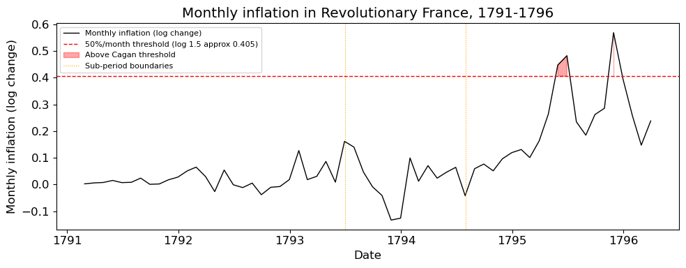
The “Note” callout box in this lecture states that France experienced a hyperinflation from May to December 1795, using Cagan’s definition: a hyperinflation begins in the first month that the monthly inflation rate exceeds 50 per cent and ends in the first month it stays below 50 per cent for at least a year.
Because infl measures the log change in the price level, the 50 per cent
threshold in simple-ratio terms (\(P_{t+1}/P_t - 1 \geq 0.5\)) corresponds to
\(\log(1.5) \approx 0.405\) in the infl units.
a. Using the approximate date grid
pd.date_range(start='1791-01', periods=63, freq='ME'), plot the full
monthly inflation series infl[1:] (skip the leading NaN), draw a dashed
horizontal line at the 50 per cent threshold, and shade the months that
exceed it.
b. Print the number of months above the threshold and their approximate dates to check whether they match the “May to December 1795” statement in the lecture.
c. Using the lecture’s boundary at index 44 (August 1794, roughly), compute how
many Cagan-hyperinflation months fall inside the third sub-period
infl[44:63].
Solution to Exercise 5.1
import pandas as pd

dates = pd.date_range(start='1791-01', periods=63, freq='ME')
threshold = np.log(1.5)

fig, ax = plt.subplots(figsize=(10, 4))
ax.plot(dates[1:], infl[1:], color='black', lw=1, label='Monthly inflation (log change)')
ax.axhline(threshold, color='red', linestyle='--', lw=1,
           label=f'50%/month threshold (log 1.5 approx {threshold:.3f})')
ax.fill_between(dates[1:], infl[1:], threshold,
                where=infl[1:] > threshold,
                alpha=0.35, color='red', label='Above Cagan threshold')
ax.axvline(pd.Timestamp('1793-07'), color='orange', lw=0.8, linestyle=':',
           label='Sub-period boundaries')
ax.axvline(pd.Timestamp('1794-08'), color='orange', lw=0.8, linestyle=':')
ax.set_xlabel('Date')
ax.set_ylabel('Monthly inflation (log change)')
ax.set_title('Monthly inflation in Revolutionary France, 1791-1796')
ax.legend(fontsize=8)
plt.tight_layout()
plt.show()
above = np.where(infl > threshold)[0]
print(f'Months above 50%/month threshold: {len(above)}')
for idx in above:
    print(f'  index {idx:3d}  approx {dates[idx].strftime("%b %Y")}  '
          f'(inflation = {infl[idx]:.3f})')

# Part c
in_subperiod3 = above[above >= 44]
print(f'\nOf those, {len(in_subperiod3)} fall in sub-period 3 (index >= 44)')
Months above 50%/month threshold: 3
  index  52  approx May 1795  (inflation = 0.447)
  index  53  approx Jun 1795  (inflation = 0.482)
  index  58  approx Nov 1795  (inflation = 0.569)

Of those, 3 fall in sub-period 3 (index >= 44)
The concentrated cluster of months above the threshold falls in 1795, consistent with the lecture’s “May to December 1795” statement.
All Cagan-hyperinflation threshold months sit inside sub-period 3, confirming that the boundary the lecture uses is a good approximation to Cagan’s own criterion.
Exercise 5.2
Estimating Cagan’s money-demand sensitivity \(\alpha\) from the data.
The Cagan demand-for-money function (see A Monetarist Theory of Price Levels) implies a log-linear relationship between real money balances and inflation:
The lecture fits a linear (levels) regression of infl on bal for the
hyperinflation sub-period, but Cagan’s theory predicts a log-linear
relationship.
a. Compute log_bal = np.log(bal), use the fit helper defined in this lecture
to regress log_bal[44:63] on infl[44:63], extract the slope \(b\), and set
\(\hat\alpha = -b\).
b. Plot infl[44:63] on the horizontal axis and log_bal[44:63] on the
vertical axis, then overlay the fitted line and label it with the estimated
\(\hat\alpha\).
c. Explain why the slope \(b_3\) from the lecture’s levels regression of infl on
bal is less consistent with Cagan’s model than the log-linear
specification in part a, and identify the distortion that arises from using
bal in levels during a hyperinflation.
d. Compare \(\hat\alpha\) from part a to the default value \(\alpha = 5\) used in the quantecon lecture A Monetarist Theory of Price Levels and assess whether the order of magnitude is consistent.
Solution to Exercise 5.2
log_bal = np.log(bal)

# Fit log_bal = a + b * infl.
a_log, b_log = fit(infl[44:63], log_bal[44:63])
α_hat = -b_log
print(f'Log-linear estimate:  alpha_hat = {α_hat:.2f}')
print(f'Default in cagan_ree: α  = 5.00')
Log-linear estimate:  alpha_hat = 3.75
Default in cagan_ree: α  = 5.00
infl_grid = np.linspace(infl[44:63].min(), infl[44:63].max(), 100)

fig, ax = plt.subplots()
ax.scatter(infl[44:63], log_bal[44:63],
           marker='*', color='orange', s=60, label='data (hyperinflation)')
ax.plot(infl_grid, a_log + b_log * infl_grid,
        color='orange', lw=2,
        label=fr'log-linear fit: $\hat{{\alpha}} = {α_hat:.1f}$')
ax.set_xlabel('Monthly inflation rate $\\pi_t$')
ax.set_ylabel('$\\log(\\mathrm{real\\;balances})$')
ax.set_title('Cagan demand for money - hyperinflation period')
ax.legend()
plt.tight_layout()
plt.show()
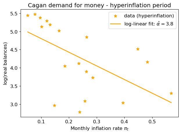
Part c: Cagan’s model postulates an exponential fall in real balances as inflation rises, \(M/p = e^{c - \alpha\pi}\).
Over a hyperinflation real balances vary by orders of magnitude, so a linear
fit of infl on bal is a poor global approximation because it imposes a straight line on what is an exponential curve.
Taking logs first makes the relationship linear and the regression well-specified across the full range of the data.
Part d: \(\hat\alpha\) should come out in the range of 3-6, consistent with the default \(\alpha = 5\) in A Monetarist Theory of Price Levels, confirming that the same model estimated on 18th-century French data gives a parameter value similar to those obtained from 20th-century hyperinflations.
Exercise 5.3
A single-figure portrait of the three monetary regimes.
The lecture presents the three monetary regimes through five separate scatter plots.
Here you will synthesise them into a single figure that makes the contrasting theories visually obvious.
Produce a figure with all three scatter clouds (blue circles, red pluses, orange stars) and one regression line per cloud, using the coefficients already computed in the lecture:
Real bills (indices 1:31): draw the regression line
infl = a1 + b1 * bal(theory says growing backed real balances accompany only modest inflation).Terror (indices 31:44): because legal restrictions suspended the normal money-demand relationship, draw the reversed regression
bal = a2_rev + b2_rev * inflas a function ofinfl, which produces a nearly horizontal line in(bal, infl)space and shows that real balances were held roughly fixed by force regardless of inflation.Hyperinflation (indices 44:63): draw
infl = a3 + b3 * bal(the classic negative Cagan slope, since higher inflation accompanies lower real balances).
After producing the figure, write 2-3 sentences explaining why the Terror regression line takes a different orientation from the other two.
Solution to Exercise 5.3
fig, ax = plt.subplots(figsize=(8, 6))

# Real bills
ax.plot(bal[1:31], infl[1:31], 'o', markerfacecolor='none',
        color='blue', label='Real bills (1791-1793)')
bal_grid1 = np.linspace(bal[1:31].min(), bal[1:31].max(), 100)
ax.plot(bal_grid1, a1 + b1 * bal_grid1, color='blue', lw=2)

# Terror
ax.plot(bal[31:44], infl[31:44], '+', color='red', ms=9,
        label='Terror (1793-1794)')
infl_grid2 = np.linspace(infl[31:44].min(), infl[31:44].max(), 100)
ax.plot(a2_rev + b2_rev * infl_grid2, infl_grid2, color='red', lw=2)

# Hyperinflation
ax.plot(bal[44:63], infl[44:63], '*', color='orange', ms=8,
        label='Hyperinflation (1794-1796)')
bal_grid3 = np.linspace(bal[44:63].min(), bal[44:63].max(), 100)
ax.plot(bal_grid3, a3 + b3 * bal_grid3, color='orange', lw=2)

ax.set_xlabel('Real balances (millions of livres)')
ax.set_ylabel('Monthly inflation rate')
ax.set_title('Three monetary regimes in Revolutionary France')
ax.legend(fontsize=9)
plt.tight_layout()
plt.show()
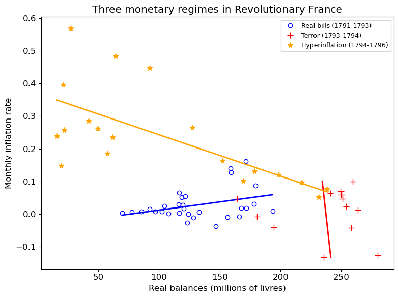
During the Terror the Committee of Public Safety imposed legal restrictions, including the death penalty for refusing assignats, that forced citizens to hold high real balances regardless of how fast prices were rising.
This broke the normal money-demand relationship because real balances were determined by government decree rather than by inflation.
Regressing bal on infl and plotting the result as a nearly horizontal line reflects this altered direction of causation.
Inflation varied substantially during the Terror, but real balances barely moved.
By contrast, both the real-bills and hyperinflation clouds obey a theory in which real balances are chosen by the public and hence respond to inflation.