13. Tax Smoothing#
13.1. Overview#
This is a sister lecture to our lecture on consumption-smoothing.
By renaming variables, we obtain a version of a model “tax-smoothing model” that Robert Barro [Barro, 1979] used to explain why governments sometimes choose not to balance their budgets every period but instead issue debt to smooth tax rates over time.
The government chooses a tax collection path that minimizes the present value of its costs of raising revenue.
The government minimizes those costs by smoothing tax collections over time and by issuing government debt during temporary surges in government expenditures.
The present value of government expenditures is at the core of the tax-smoothing model, so we’ll again use formulas presented in present value formulas.
We’ll again use the matrix multiplication and matrix inversion tools that we used in present value formulas.
13.2. Analysis#
As usual, we’ll start by importing some Python modules.
import numpy as np
import matplotlib.pyplot as plt
from collections import namedtuple
A government exists at times \(t=0, 1, \ldots, S\) and faces an exogenous stream of expenditures \(\{G_t\}_{t=0}^S\).
It chooses a stream of tax collections \(\{T_t\}_{t=0}^S\).
The model takes a government expenditure stream as an “exogenous” input that is somehow determined outside the model.
The government faces a gross interest rate of \(R >1\) that is constant over time.
The government can borrow or lend at interest rate \(R\), subject to some limits on the amount of debt that it can issue that we’ll describe below.
Let
\(S \geq 2\) be a positive integer that constitutes a time-horizon.
\(G = \{G_t\}_{t=0}^S\) be a sequence of government expenditures.
\(B = \{B_t\}_{t=0}^{S+1}\) be a sequence of government debt.
\(T = \{T_t\}_{t=0}^S\) be a sequence of tax collections.
\(R \geq 1\) be a fixed gross one period interest rate.
\(\beta \in (0,1)\) be a fixed discount factor.
\(B_0\) be a given initial level of government debt
\(B_{S+1} \geq 0\) be a terminal condition.
The sequence of government debt \(B\) is to be determined by the model.
We require it to satisfy two boundary conditions:
it must equal an exogenous value \(B_0\) at time \(0\)
it must equal or exceed an exogenous value \(B_{S+1}\) at time \(S+1\).
The terminal condition \(B_{S+1} \geq 0\) requires that the government not end up with negative assets.
(This no-Ponzi condition ensures that the government ultimately pays off its debts – it can’t simply roll them over indefinitely.)
The government faces a sequence of budget constraints that constrain sequences \((G, T, B)\)
Equations (13.1) constitute \(S+1\) such budget constraints, one for each \(t=0, 1, \ldots, S\).
Given a sequence \(G\) of government expenditures, a large set of pairs \((B, T)\) of (government debt, tax collections) sequences satisfy the sequence of budget constraints (13.1).
The model follows the following logical flow:
start with an exogenous government expenditure sequence \(G\), an initial government debt \(B_0\), and a candidate tax collection path \(T\).
use the system of equations (13.1) for \(t=0, \ldots, S\) to compute a path \(B\) of government debt
verify that \(B_{S+1}\) satisfies the terminal debt constraint \(B_{S+1} \geq 0\).
If it does, declare that the candidate path is budget feasible.
if the candidate tax path is not budget feasible, propose a different tax path and start over
Below, we’ll describe how to execute these steps using linear algebra – matrix inversion and multiplication.
The above procedure seems like a sensible way to find “budget-feasible” tax paths \(T\), i.e., paths that are consistent with the exogenous government expenditure stream \(G\), the initial debt level \(B_0\), and the terminal debt level \(B_{S+1}\).
In general, there are many budget feasible tax paths \(T\).
Among all budget-feasible tax paths, which one should a government choose?
To answer this question, we assess alternative budget feasible tax paths \(T\) using the following cost functional:
where \(g_1 > 0, g_2 > 0\).
This is called the “present value of revenue-raising costs” in [Barro, 1979].
The quadratic term \(-\frac{g_2}{2} T_t^2\) captures increasing marginal costs of taxation, implying that tax distortions rise more than proportionally with tax rates.
This creates an incentive for tax smoothing.
Indeed, we shall see that when \(\beta R = 1\), criterion (13.2) leads to smoother tax paths.
By smoother we mean tax rates that are as close as possible to being constant over time.
The preference for smooth tax paths that is built into the model gives it the name “tax-smoothing model”.
Or equivalently, we can transform this into the same problem as in the consumption-smoothing lecture by maximizing the welfare criterion:
Let’s dive in and do some calculations that will help us understand how the model works.
Here we use default parameters \(R = 1.05\), \(g_1 = 1\), \(g_2 = 1/2\), and \(S = 65\).
We create a Python namedtuple to store these parameters with default values.
TaxSmoothing = namedtuple("TaxSmoothing",
                        ["R", "g1", "g2", "β_seq", "S"])

def create_tax_smoothing_model(R=1.01, g1=1, g2=1/2, S=65):
    """
    Creates an instance of the tax smoothing model.
    """
    β = 1/R
    β_seq = np.array([β**i for i in range(S+1)])

    return TaxSmoothing(R, g1, g2, β_seq, S)
13.3. Barro tax-smoothing model#
A key object is the present value of government expenditures at time \(0\):
This sum represents the present value of all future government expenditures that must be financed.
Formally it resembles the present value calculations we saw in this QuantEcon lecture present values.
This present value calculation is crucial for determining the government’s total financing needs.
By iterating on equation (13.1) and imposing the terminal condition
it is possible to convert a sequence of budget constraints (13.1) into a single intertemporal constraint
Equation (13.4) says that the present value of tax collections must equal the sum of initial debt and the present value of government expenditures.
When \(\beta R = 1\), it is optimal for a government to smooth taxes by setting
(Later we’ll present a “variational argument” that shows that this constant path minimizes criterion (13.2) and maximizes (13.3) when \(\beta R =1\).)
In this case, we can use the intertemporal budget constraint to write
Equation (13.5) is the tax-smoothing model in a nutshell.
13.4. Mechanics of tax-smoothing#
As promised, we’ll provide step-by-step instructions on how to use linear algebra, readily implemented in Python, to compute all objects in play in the tax-smoothing model.
In the calculations below, we’ll set default values of \(R > 1\), e.g., \(R = 1.05\), and \(\beta = R^{-1}\).
13.4.1. Step 1#
For a \((S+1) \times 1\) vector \(G\) of government expenditures, use matrix algebra to compute the present value
13.4.2. Step 2#
Compute a constant tax rate \(T_0\):
13.4.3. Step 3#
Use the system of equations (13.1) for \(t=0, \ldots, S\) to compute a path \(B\) of government debt.
To do this, we transform that system of difference equations into a single matrix equation as follows:
Multiply both sides by the inverse of the matrix on the left side to compute
Because we have built into our calculations that the government must satisfy its intertemporal budget constraint and end with zero debt, just barely satisfying the terminal condition that \(B_{S+1} \geq 0\), it should turn out that
Let’s verify this with Python code.
First we implement the model with compute_optimal
def compute_optimal(model, B0, G_seq):

    R, S = model.R, model.S

    # present value of government expenditures
    h0 = model.β_seq @ G_seq     # since β = 1/R

    # optimal constant tax rate
    T0 = (1 - 1/R) / (1 - (1/R)**(S+1)) * (B0 + h0)
    T_seq = T0*np.ones(S+1)

    A = np.diag(-R*np.ones(S), k=-1) + np.eye(S+1)
    b = G_seq - T_seq
    b[0] = b[0] + B0
    B_seq = np.linalg.inv(A) @ (R * b)
    B_seq = np.concatenate([[B0], B_seq])

    return T_seq, B_seq, h0
We use an example where the government starts with initial debt \(B_0>0\).
This represents the government’s initial debt burden.
The government expenditure process \(\{G_t\}_{t=0}^{S}\) is constant and positive up to \(t=45\) and then drops to zero afterward.
The drop in government expenditures could reflect a change in spending requirements or demographic shifts.
# Initial debt
B0 = 2     # initial government debt

# Government expenditure process
G_seq = np.concatenate([np.ones(46), 4*np.ones(5), np.ones(15)])
tax_model = create_tax_smoothing_model()
T_seq, B_seq, h0 = compute_optimal(tax_model, B0, G_seq)

print('check B_S+1=0:',
      np.abs(B_seq[-1] - 0) <= 1e-8)
check B_S+1=0: True
The graphs below show paths of government expenditures, tax collections, and government debt.
# Sequence length
S = tax_model.S

fig, axes = plt.subplots(1, 2, figsize=(12,5))

axes[0].plot(range(S+1), G_seq, label='expenditures', lw=2)
axes[0].plot(range(S+1), T_seq, label='tax', lw=2)
axes[1].plot(range(S+2), B_seq, label='debt', color='green', lw=2)
axes[0].set_ylabel(r'$T_t,G_t$')
axes[1].set_ylabel(r'$B_t$')

for ax in axes:
    ax.plot(range(S+2), np.zeros(S+2), '--', lw=1, color='black')
    ax.legend()
    ax.set_xlabel(r'$t$')

plt.show()
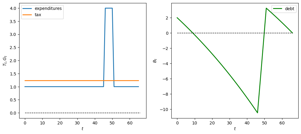
Note that \(B_{S+1} = 0\), as anticipated.
We can evaluate cost criterion (13.2) which measures the total cost / welfare of taxation
def cost(model, T_seq):
    β_seq, g1, g2 = model.β_seq, model.g1, model.g2
    cost_seq = g1 * T_seq - g2/2 * T_seq**2
    return - β_seq @ cost_seq

print('Cost:', cost(tax_model, T_seq))

def welfare(model, T_seq):
    return - cost(model, T_seq)

print('Welfare:', welfare(tax_model, T_seq))
Cost: -41.46532630469102
Welfare: 41.46532630469102
13.4.4. Experiments#
In this section we describe how a tax sequence would optimally respond to different sequences of government expenditures.
First we create a function plot_ts that generates graphs for different instances of the tax-smoothing model tax_model.
This will help us avoid rewriting code to plot outcomes for different government expenditure sequences.
def plot_ts(model,    # tax-smoothing model
            B0,       # initial government debt
            G_seq     # government expenditure process
           ):

    # Compute optimal tax path
    T_seq, B_seq, h0 = compute_optimal(model, B0, G_seq)

    # Sequence length
    S = model.S

    fig, axes = plt.subplots(1, 2, figsize=(12,5))

    axes[0].plot(range(S+1), G_seq, label='expenditures', lw=2)
    axes[0].plot(range(S+1), T_seq, label='taxes', lw=2)
    axes[1].plot(range(S+2), B_seq, label='debt', color='green', lw=2)
    axes[0].set_ylabel(r'$T_t,G_t$')
    axes[1].set_ylabel(r'$B_t$')

    for ax in axes:
        ax.plot(range(S+2), np.zeros(S+2), '--', lw=1, color='black')
        ax.legend()
        ax.set_xlabel(r'$t$')


    plt.show()
In the experiments below, please study how tax and government debt sequences vary across different sequences for government expenditures.
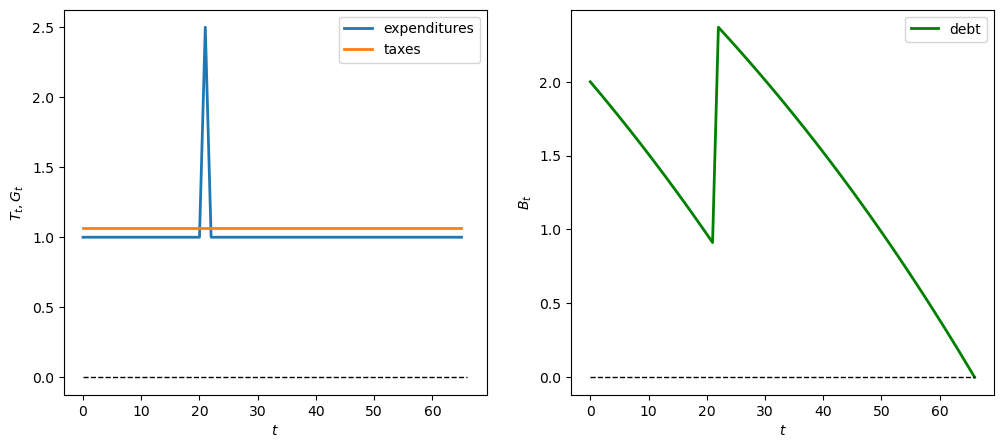
13.4.4.1. Experiment 1: one-time spending shock#
We first assume a one-time spending shock of \(W_0\) in year 21 of the expenditure sequence \(G\).
We’ll make \(W_0\) big - positive to indicate a spending surge (like a war or disaster), and negative to indicate a spending cut.
# Spending surge W_0 = 2.5
G_seq_pos = np.concatenate([np.ones(21), np.array([2.5]),
np.ones(24), np.ones(20)])

plot_ts(tax_model, B0, G_seq_pos)
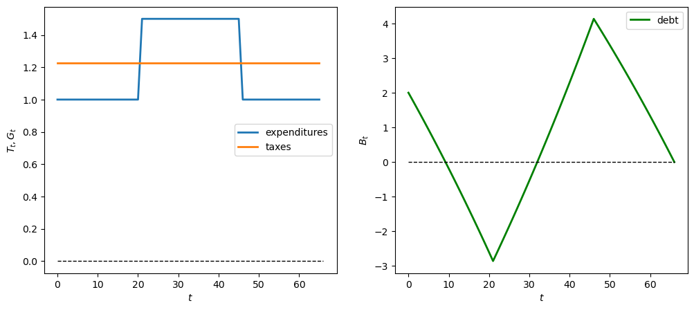
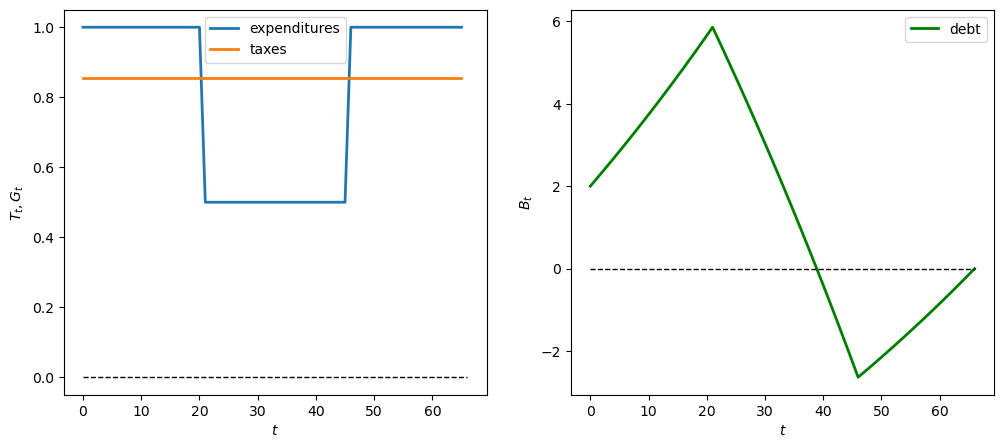
13.4.4.2. Experiment 2: temporary expenditure shift#
Now we assume a temporary increase in government expenditures of \(L\) beginning in year 21 of the \(G\)-sequence.
Again we can study positive and negative cases
# Positive temporary expenditure shift L = 0.5 when t >= 21
G_seq_pos = np.concatenate(
    [np.ones(21), 1.5*np.ones(25), np.ones(20)])

plot_ts(tax_model, B0, G_seq_pos)
# Negative temporary expenditure shift L = -0.5 when t >= 21
G_seq_neg = np.concatenate(
    [np.ones(21), .5*np.ones(25), np.ones(20)])

plot_ts(tax_model, B0, G_seq_neg)
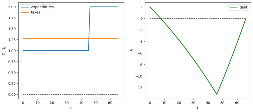
13.4.4.3. Experiment 3: delayed spending surge#
Now we simulate a \(G\) sequence in which government expenditures are zero for 46 years, and then rise to 1 for the last 20 years (perhaps due to demographic aging)
# Delayed spending
G_seq_late = np.concatenate(
    [np.ones(46), 2*np.ones(20)])

plot_ts(tax_model, B0, G_seq_late)
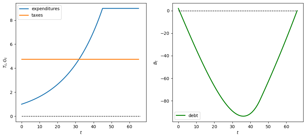
13.4.4.4. Experiment 4: growing expenditures#
Now we simulate a geometric \(G\) sequence in which government expenditures grow at rate \(G_t = \lambda^t G_0\) in first 46 years.
We first experiment with \(\lambda = 1.05\) (growing expenditures)
# Geometric growth parameters where λ = 1.05
λ = 1.05
G_0 = 1
t_max = 46

# Generate geometric G sequence
geo_seq = λ ** np.arange(t_max) * G_0
G_seq_geo = np.concatenate(
            [geo_seq, np.max(geo_seq)*np.ones(20)])

plot_ts(tax_model, B0, G_seq_geo)
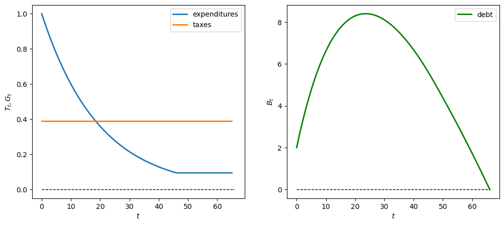
Now we show the behavior when \(\lambda = 0.95\) (declining expenditures)
λ = 0.95
geo_seq = λ ** np.arange(t_max) * G_0
G_seq_geo = np.concatenate(
            [geo_seq, λ ** t_max * np.ones(20)])

plot_ts(tax_model, B0, G_seq_geo)
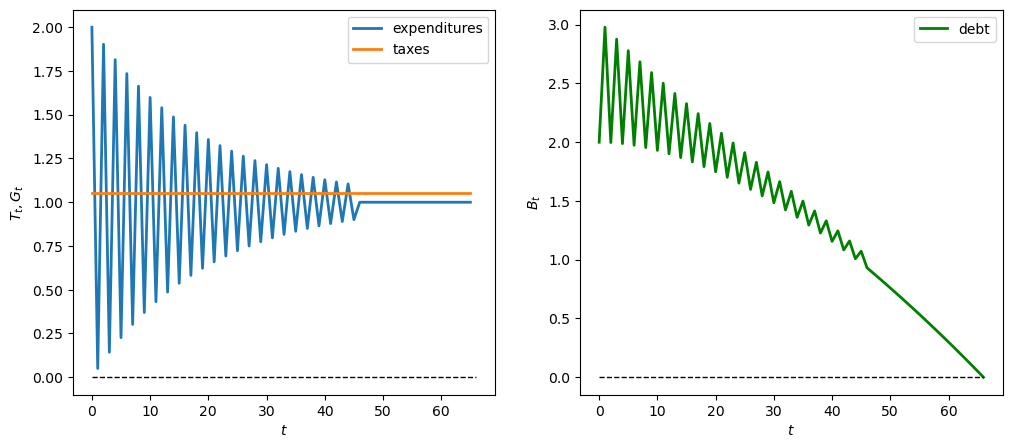
What happens with oscillating expenditures
λ = -0.95
geo_seq = λ ** np.arange(t_max) * G_0 + 1
G_seq_geo = np.concatenate(
            [geo_seq, np.ones(20)])

plot_ts(tax_model, B0, G_seq_geo)
13.4.5. Feasible Tax Variations#
We promised to justify our claim that a constant tax rate \(T_t = T_0\) for all \(t\) is optimal.
Let’s do that now.
The approach we’ll take is an elementary example of the “calculus of variations”.
Let’s dive in and see what the key idea is.
To explore what types of tax paths are cost-minimizing / welfare-improving, we shall create an admissible tax path variation sequence \(\{v_t\}_{t=0}^S\) that satisfies
This equation says that the present value of admissible tax path variations must be zero.
So once again, we encounter a formula for the present value:
we require that the present value of tax path variations be zero to maintain budget balance.
Here we’ll restrict ourselves to a two-parameter class of admissible tax path variations of the form
We say two and not three-parameter class because \(\xi_0\) will be a function of \((\phi, \xi_1; R)\) that guarantees that the variation sequence is feasible.
Let’s compute that function.
We require
which implies that
which implies that
which implies that
This is our formula for \(\xi_0\).
Key Idea: if \(T^o\) is a budget-feasible tax path, then so is \(T^o + v\), where \(v\) is a budget-feasible variation.
Given \(R\), we thus have a two parameter class of budget feasible variations \(v\) that we can use to compute alternative tax paths, then evaluate their welfare costs.
Now let’s compute and plot tax path variations
def compute_variation(model, ξ1, ϕ, B0, G_seq, verbose=1):
    R, S, β_seq = model.R, model.S, model.β_seq

    ξ0 = ξ1*((1 - 1/R) / (1 - (1/R)**(S+1))) * ((1 - (ϕ/R)**(S+1)) / (1 - ϕ/R))
    v_seq = np.array([(ξ1*ϕ**t - ξ0) for t in range(S+1)])

    if verbose == 1:
        print('check feasible:', np.isclose(β_seq @ v_seq, 0))

    T_opt, _, _ = compute_optimal(model, B0, G_seq)
    Tvar_seq = T_opt + v_seq

    return Tvar_seq
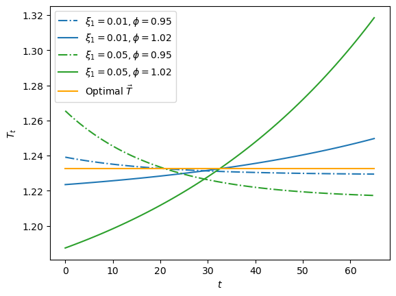
We visualize variations for \(\xi_1 \in \{.01, .05\}\) and \(\phi \in \{.95, 1.02\}\)
fig, ax = plt.subplots()
ξ1s = [.01, .05]
ϕs= [.95, 1.02]
colors = {.01: 'tab:blue', .05: 'tab:green'}
params = np.array(np.meshgrid(ξ1s, ϕs)).T.reshape(-1, 2)
wel_opt = welfare(tax_model, T_seq)

for i, param in enumerate(params):
    ξ1, ϕ = param
    print(f'variation {i}: ξ1={ξ1}, ϕ={ϕ}')

    Tvar_seq = compute_variation(model=tax_model,
                                 ξ1=ξ1, ϕ=ϕ, B0=B0,
                                 G_seq=G_seq)
    print(f'welfare={welfare(tax_model, Tvar_seq)}')
    print(f'welfare < optimal: {welfare(tax_model, Tvar_seq) < wel_opt}')
    print('-'*64)

    if i % 2 == 0:
        ls = '-.'
    else:
        ls = '-'
    ax.plot(range(S+1), Tvar_seq, ls=ls,
            color=colors[ξ1],
            label=fr'$\xi_1 = {ξ1}, \phi = {ϕ}$')

plt.plot(range(S+1), T_seq,
         color='orange', label=r'Optimal $\vec{T}$ ')

plt.legend()
plt.xlabel(r'$t$')
plt.ylabel(r'$T_t$')
plt.show()
variation 0: ξ1=0.01, ϕ=0.95
check feasible: True
welfare=41.46523217108914
welfare < optimal: True
----------------------------------------------------------------
variation 1: ξ1=0.01, ϕ=1.02
check feasible: True
welfare=41.46467728803246
welfare < optimal: True
----------------------------------------------------------------
variation 2: ξ1=0.05, ϕ=0.95
check feasible: True
welfare=41.46297296464396
welfare < optimal: True
----------------------------------------------------------------
variation 3: ξ1=0.05, ϕ=1.02
check feasible: True
welfare=41.44910088822694
welfare < optimal: True
----------------------------------------------------------------
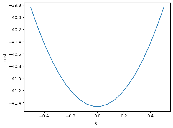
We can even use the Python np.gradient command to compute derivatives of cost with respect to our two parameters.
We are teaching the key idea beneath the calculus of variations. First, we define the cost with respect to \(\xi_1\) and \(\phi\)
def cost_rel(ξ1, ϕ):
    """
    Compute cost of variation sequence
    for given ϕ, ξ1 with a tax-smoothing model
    """

    Tvar_seq = compute_variation(tax_model, ξ1=ξ1,
                                 ϕ=ϕ, B0=B0,
                                 G_seq=G_seq,
                                 verbose=0)
    return cost(tax_model, Tvar_seq)

# Vectorize the function to allow array input
cost_vec = np.vectorize(cost_rel)
Then we can visualize the relationship between cost and \(\xi_1\) and compute its derivatives
ξ1_arr = np.linspace(-0.5, 0.5, 20)
plt.plot(ξ1_arr, cost_vec(ξ1_arr, 1.02))
plt.ylabel('cost')
plt.xlabel(r'$\xi_1$')
plt.show()
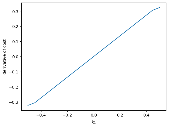
cost_grad = cost_vec(ξ1_arr, 1.02)
cost_grad = np.gradient(cost_grad)
plt.plot(ξ1_arr, cost_grad)
plt.ylabel('derivative of cost')
plt.xlabel(r'$\xi_1$')
plt.show()
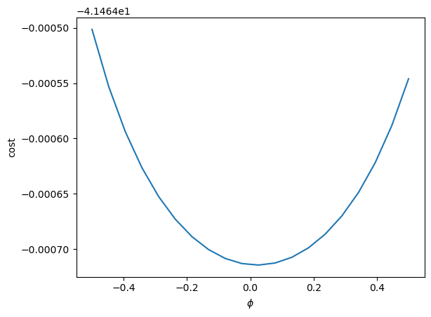
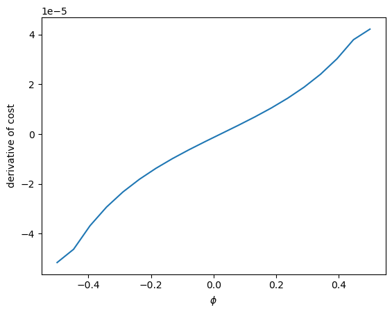
The same can be done on \(\phi\)
ϕ_arr = np.linspace(-0.5, 0.5, 20)

plt.plot(ξ1_arr, cost_vec(0.05, ϕ_arr))
plt.ylabel('cost')
plt.xlabel(r'$\phi$')
plt.show()

cost_grad = cost_vec(0.05, ϕ_arr)
cost_grad = np.gradient(cost_grad)
plt.plot(ϕ_arr, cost_grad)
plt.ylabel('derivative of cost')
plt.xlabel(r'$\phi$')
plt.show()
13.5. Exercises#
Exercise 13.1
For the default expenditure sequence and \(B_0 = 0\), suppose a one-time spending spike of size \(W_0 = 1\) occurs at period \(t^* = 20\).
a. Compute the optimal constant tax rate \(T_0\) for the baseline expenditure sequence (without the spike) and for the sequence with the spike, then print the difference \(\Delta T_0\).
b. The present value of the spike is \(W_0 R^{-t^*}\). Show analytically that the increase in the optimal flat tax equals the annuity value of that present value:
$$
\Delta T_0 = \left(\frac{1 - R^{-1}}{1 - R^{-(S+1)}}\right) W_0 R^{-t^*}
$$

Verify numerically that the formula matches the computed $\Delta T_0$.
Solution to Exercise 13.1
tax_model = create_tax_smoothing_model()
S, R = tax_model.S, tax_model.R
B0 = 0

G_base = np.concatenate([np.ones(46), 4*np.ones(5), np.ones(15)])
T_base, _, _ = compute_optimal(tax_model, B0, G_base)

t_star = 20
W0 = 1.0
G_shock = G_base.copy()
G_shock[t_star] += W0
T_shock, _, _ = compute_optimal(tax_model, B0, G_shock)

delta_T0_numerical = T_shock[0] - T_base[0]

annuity_factor = (1 - 1/R) / (1 - (1/R)**(S+1))
delta_T0_formula = annuity_factor * W0 * R**(-t_star)

print(f'Numerical ΔT0:           {delta_T0_numerical:.10f}')
print(f'Annuity-value formula:   {delta_T0_formula:.10f}')
print(f'Match: {np.isclose(delta_T0_numerical, delta_T0_formula)}')
Numerical ΔT0:           0.0168538277
Annuity-value formula:   0.0168538277
Match: True
The spike raises \(h_0\), the present value of expenditures, by exactly \(W_0 R^{-t^*}\).
Since the optimal flat tax is the annuity value of \((B_0 + h_0)\), the increase in \(T_0\) is the annuity value of the extra present-value cost.
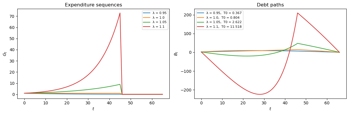
Exercise 13.2
Using compute_optimal, compute the optimal flat tax \(T_0\) for four geometrically
growing expenditure paths \(G_t = \lambda^t G_0\) (for the working years
\(t = 0, \ldots, 45\), then \(G_t = 0\) thereafter), with \(G_0 = 1\) and
\(\lambda \in \{0.95,\, 1.00,\, 1.05,\, 1.10\}\).
a. Plot the four expenditure sequences on one set of axes and the corresponding debt paths \(B_t\) on a second set.
b. Identify which \(\lambda\) requires the highest flat tax and explain why in terms of the present-value formula for \(h_0\).
Solution to Exercise 13.2
tax_model = create_tax_smoothing_model()
S = tax_model.S
B0 = 2
t_max = 46
λ_vals = [0.95, 1.00, 1.05, 1.10]

fig, axes = plt.subplots(1, 2, figsize=(12, 4))

for λ in λ_vals:
    G_seq = np.concatenate(
        [λ**np.arange(t_max), np.zeros(S + 1 - t_max)])
    T_seq, B_seq, _ = compute_optimal(tax_model, B0, G_seq)
    axes[0].plot(range(S+1), G_seq, label=f'λ = {λ}')
    axes[1].plot(range(S+2), B_seq,
                 label=f'λ = {λ},  T0 = {T_seq[0]:.3f}')

for ax in axes:
    ax.legend(fontsize=8)
    ax.set_xlabel('$t$')
axes[0].set_ylabel('$G_t$')
axes[0].set_title('Expenditure sequences')
axes[1].set_ylabel('$B_t$')
axes[1].set_title('Debt paths')

plt.tight_layout()
plt.show()

print(f"{'λ':>6} | {'T0':>10} | {'h0':>12}")
print('-' * 34)
for λ in λ_vals:
    G_seq = np.concatenate(
        [λ**np.arange(t_max), np.zeros(S + 1 - t_max)])
    T_seq, _, h0 = compute_optimal(tax_model, B0, G_seq)
    print(f'{λ:>6.2f} | {T_seq[0]:>10.4f} | {h0:>12.4f}')
     λ |         T0 |           h0
----------------------------------
  0.95 |     0.3666 |      15.8272
  1.00 |     0.8040 |      37.0945
  1.05 |     2.6215 |     125.4752
  1.10 |    11.5184 |     558.1014
Faster spending growth, or a higher \(\lambda\), leaves initial spending unchanged but raises later spending enough to increase the present value \(h_0\) despite discounting.
A higher \(h_0\) translates directly into a higher required flat tax.
Exercise 13.3
Show numerically that the constant (optimal) tax path yields strictly lower cost (13.2), equivalently, strictly higher welfare (13.3), than any non-constant budget-feasible tax path.
Use the default expenditure sequence and \(B_0 = 2\) to evaluate welfare for the
optimal flat path and for four variations generated by compute_variation with
\((\xi_1, \phi) \in \{(0.2, 0.95),\, (0.2, 1.05),\, (-0.2, 0.90),\, (-0.2, 1.10)\}\),
then print a table showing each path’s welfare and its gap relative to the optimum.
Solution to Exercise 13.3
tax_model = create_tax_smoothing_model()
S = tax_model.S
B0 = 2
G_seq = np.concatenate([np.ones(46), 4*np.ones(5), np.ones(15)])

T_seq, _, _ = compute_optimal(tax_model, B0, G_seq)
w_opt = welfare(tax_model, T_seq)

print(f'Optimal (flat) welfare: {w_opt:.6f}\n')

params = [(0.2, 0.95), (0.2, 1.05), (-0.2, 0.90), (-0.2, 1.10)]
print(f'{"ξ1":>6} | {"ϕ":>6} | {"welfare":>12} | {"gap":>14}')
print('-' * 46)
for ξ1, ϕ in params:
    Tvar = compute_variation(tax_model, ξ1=ξ1, ϕ=ϕ,
                             B0=B0, G_seq=G_seq, verbose=0)
    w = welfare(tax_model, Tvar)
    print(f'{ξ1:>6.2f} | {ϕ:>6.2f} | {w:>12.6f} | {w - w_opt:>+14.6f}')
Optimal (flat) welfare: 41.465326

    ξ1 |      ϕ |      welfare |            gap
----------------------------------------------
  0.20 |   0.95 |    41.427673 |      -0.037653
  0.20 |   1.05 |    24.915043 |     -16.550284
 -0.20 |   0.90 |    41.432147 |      -0.033180
 -0.20 |   1.10 | -5565.980135 |   -5607.445462
Every variation yields strictly lower welfare, or a more negative gap, than the flat path.
This confirms that the constant tax schedule is the global welfare maximiser under the quadratic criterion (13.3) when \(\beta R = 1\).
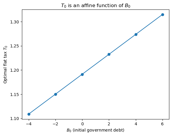
Exercise 13.4
Show that the optimal flat tax \(T_0\) is an affine (linear) function of initial government debt \(B_0\).
For the default expenditure sequence \(G\), compute \(T_0\) for \(B_0 \in \{-4, -2, 0, 2, 4, 6\}\), plot \(T_0\) against \(B_0\), and verify that the slope equals the annuity factor \(\left(\frac{1-R^{-1}}{1-R^{-(S+1)}}\right)\).
Solution to Exercise 13.4
tax_model = create_tax_smoothing_model()
S, R = tax_model.S, tax_model.R
G_seq = np.concatenate([np.ones(46), 4*np.ones(5), np.ones(15)])

B0_vals = [-4, -2, 0, 2, 4, 6]
T0_vals = []

for B0 in B0_vals:
    T_seq, _, _ = compute_optimal(tax_model, B0, G_seq)
    T0_vals.append(T_seq[0])

fig, ax = plt.subplots()
ax.plot(B0_vals, T0_vals, 'o-')
ax.set_xlabel('$B_0$ (initial government debt)')
ax.set_ylabel('Optimal flat tax $T_0$')
ax.set_title('$T_0$ is an affine function of $B_0$')
plt.show()

slope = (T0_vals[-1] - T0_vals[0]) / (B0_vals[-1] - B0_vals[0])
annuity = (1 - 1/R) / (1 - (1/R)**(S+1))
print(f'Numerical slope of T0 w.r.t. B0: {slope:.8f}')
print(f'Annuity factor:                   {annuity:.8f}')
print(f'Match: {np.isclose(slope, annuity)}')
Numerical slope of T0 w.r.t. B0: 0.02056487
Annuity factor:                   0.02056487
Match: True
From equation (13.5), \(T_0 = \text{annuity factor} \times (B_0 + h_0)\).
The coefficient on \(B_0\) is exactly the annuity factor, confirming the linear relationship.
Higher initial debt forces the government to collect more tax in every period to satisfy its intertemporal budget constraint.