11. Present Values#
11.1. Overview#
This lecture describes the present value model that is a starting point of much asset pricing theory.
Asset pricing theory is a component of theories about many economic decisions including
consumption
labor supply
education choice
demand for money
In asset pricing theory, and in economic dynamics more generally, a basic topic is the relationship among different time series.
A time series is a sequence indexed by time.
In this lecture, we’ll represent a sequence as a vector.
So our analysis will typically boil down to studying relationships among vectors.
Our main tools in this lecture will be
matrix multiplication, and
matrix inversion.
We’ll use the calculations described here in subsequent lectures, including consumption smoothing, equalizing difference model, and monetarist theory of price levels.
Let’s dive in.
11.2. Analysis#
Let
\(\{d_t\}_{t=0}^T \) be a sequence of dividends or “payouts”
\(\{p_t\}_{t=0}^T \) be a sequence of prices of a claim on the continuation of the asset’s payout stream from date \(t\) on, namely, \(\{d_s\}_{s=t}^T \)
\( \delta \in (0,1) \) be a one-period “discount factor”
\(p_{T+1}^*\) be a terminal price of the asset at time \(T+1\)
We assume that the dividend stream \(\{d_t\}_{t=0}^T \) and the terminal price \(p_{T+1}^*\) are both exogenous.
This means that they are determined outside the model.
Assume the sequence of asset pricing equations
We say equations, plural, because there are \(T+1\) equations, one for each \(t =0, 1, \ldots, T\).
Equations (11.1) assert that price paid to purchase the asset at time \(t\) equals the payout \(d_t\) plus the price at time \(t+1\) multiplied by a time discount factor \(\delta\).
Discounting tomorrow’s price by multiplying it by \(\delta\) accounts for the “value of waiting one period”.
We want to solve the system of \(T+1\) equations (11.1) for the asset price sequence \(\{p_t\}_{t=0}^T \) as a function of the dividend sequence \(\{d_t\}_{t=0}^T \) and the exogenous terminal price \(p_{T+1}^*\).
A system of equations like (11.1) is an example of a linear difference equation.
There are powerful mathematical methods available for solving such systems and they are well worth studying in their own right, being the foundation for the analysis of many interesting economic models.
For an example, see Samuelson multiplier-accelerator
In this lecture, we’ll solve system (11.1) using matrix multiplication and matrix inversion, basic tools from linear algebra introduced in linear equations and matrix algebra.
We will use the following imports
import numpy as np
import matplotlib.pyplot as plt
11.3. Representing sequences as vectors#
The equations in system (11.1) can be arranged as follows:
Write the system (11.2) of \(T+1\) asset pricing equations as the single matrix equation
Exercise 11.1
Carry out the matrix multiplication in (11.3) by hand and confirm that you recover the equations in (11.2).
Solution to Exercise 11.1
Multiplying row \(t\) of the matrix (which has \(1\) in column \(t\) and \(-\delta\) in column \(t+1\)) against the price vector gives \(p_t - \delta p_{t+1}\).
The last row has only a \(1\) in column \(T\), giving \(p_T\).
Setting these equal to the right-hand side recovers exactly the equations in (11.2).
We can verify the result numerically.
T = 6
δ = 0.99
p_star = 10.0
d = np.array([1.0 * 1.05**t for t in range(T+1)])

# Build A
A = np.zeros((T+1, T+1))
for i in range(T+1):
    A[i, i] = 1
    if i < T:
        A[i, i+1] = -δ

b = np.zeros(T+1)
b[-1] = δ * p_star

# Solve for p
p = np.linalg.solve(A, d + b)

# Check that A @ p == d + b  (residual should be zero)
residual = A @ p - (d + b)
print("Max residual |A p - (d + b)|:", np.max(np.abs(residual)))
Max residual |A p - (d + b)|: 1.1102230246251565e-15
In vector-matrix notation, we can write system (11.3) as
Here \(A\) is the matrix on the left side of equation (11.3), while
The solution for the vector of prices is
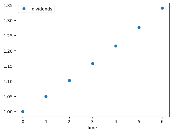
For example, suppose that the dividend stream is
Let’s write Python code to compute and plot the dividend stream.
T = 6
current_d = 1.0
d = []
for t in range(T+1):
    d.append(current_d)
    current_d = current_d * 1.05

fig, ax = plt.subplots()
ax.plot(d, 'o', label='dividends')
ax.legend()
ax.set_xlabel('time')
plt.show()
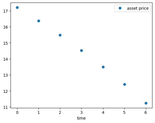
Now let’s compute and plot the asset price.
We set \(\delta\) and \(p_{T+1}^*\) to
δ = 0.99
p_star = 10.0
Let’s build the matrix \(A\)
A = np.zeros((T+1, T+1))
for i in range(T+1):
    for j in range(T+1):
        if i == j:
            A[i, j] = 1
            if j < T:
                A[i, j+1] = -δ
Let’s inspect \(A\)
A
array([[ 1.  , -0.99,  0.  ,  0.  ,  0.  ,  0.  ,  0.  ],
       [ 0.  ,  1.  , -0.99,  0.  ,  0.  ,  0.  ,  0.  ],
       [ 0.  ,  0.  ,  1.  , -0.99,  0.  ,  0.  ,  0.  ],
       [ 0.  ,  0.  ,  0.  ,  1.  , -0.99,  0.  ,  0.  ],
       [ 0.  ,  0.  ,  0.  ,  0.  ,  1.  , -0.99,  0.  ],
       [ 0.  ,  0.  ,  0.  ,  0.  ,  0.  ,  1.  , -0.99],
       [ 0.  ,  0.  ,  0.  ,  0.  ,  0.  ,  0.  ,  1.  ]])
Now let’s solve for prices using (11.5).
b = np.zeros(T+1)
b[-1] = δ * p_star
p = np.linalg.solve(A, d + b)
fig, ax = plt.subplots()
ax.plot(p, 'o', label='asset price')
ax.legend()
ax.set_xlabel('time')
plt.show()
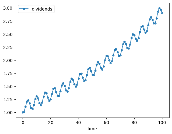
Now let’s consider a cyclically growing dividend sequence:
T = 100
current_d = 1.0
d = []
for t in range(T+1):
    d.append(current_d)
    current_d = current_d * 1.01 + 0.1 * np.sin(t)

fig, ax = plt.subplots()
ax.plot(d, 'o-', ms=4, alpha=0.8, label='dividends')
ax.legend()
ax.set_xlabel('time')
plt.show()
Exercise 11.2
Compute the corresponding asset price sequence when \(p^*_{T+1} = 0\) and \(\delta = 0.98\).
Solution to Exercise 11.2
We proceed as above after modifying parameters and consequently the matrix \(A\).
δ = 0.98
p_star = 0.0
A = np.zeros((T+1, T+1))
for i in range(T+1):
    for j in range(T+1):
        if i == j:
            A[i, j] = 1
            if j < T:
                A[i, j+1] = -δ

b = np.zeros(T+1)
b[-1] = δ * p_star
p = np.linalg.solve(A, d + b)
fig, ax = plt.subplots()
ax.plot(p, 'o-', ms=4, alpha=0.8, label='asset price')
ax.legend()
ax.set_xlabel('time')
plt.show()
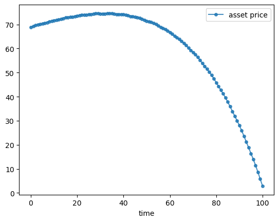
The weighted averaging associated with the present value calculation largely eliminates the cycles.
11.4. Analytical expressions#
By the inverse matrix theorem, a matrix \(B\) is the inverse of \(A\) whenever \(A B\) is the identity.
It can be verified that the inverse of the matrix \(A\) in (11.3) is
Exercise 11.3
Check this by showing that \(A A^{-1}\) is equal to the identity matrix.
Solution to Exercise 11.3
T = 6
δ = 0.99

# Build A
A = np.zeros((T+1, T+1))
for i in range(T+1):
    A[i, i] = 1
    if i < T:
        A[i, i+1] = -δ

# Analytical inverse from eq:Ainv: A_inv[i,j] = δ^(j-i) for j >= i, else 0
A_inv = np.zeros((T+1, T+1))
for i in range(T+1):
    for j in range(i, T+1):
        A_inv[i, j] = δ**(j - i)

# Verify
print("A @ A_inv (should be identity):")
print(np.round(A @ A_inv, 10))
print("Is identity:", np.allclose(A @ A_inv, np.eye(T+1)))
A @ A_inv (should be identity):
[[ 1.  0.  0.  0. -0.  0.  0.]
 [ 0.  1.  0.  0.  0. -0.  0.]
 [ 0.  0.  1.  0.  0.  0. -0.]
 [ 0.  0.  0.  1.  0.  0.  0.]
 [ 0.  0.  0.  0.  1.  0.  0.]
 [ 0.  0.  0.  0.  0.  1.  0.]
 [ 0.  0.  0.  0.  0.  0.  1.]]
Is identity: True
If we use the expression (11.6) in (11.5) and perform the indicated matrix multiplication, we shall find that
Pricing formula (11.7) asserts that two components sum to the asset price \(p_t\):
a fundamental component \(\sum_{s=t}^T \delta^{s-t} d_s\) that equals the discounted present value of prospective dividends
a bubble component \(\delta^{T+1-t} p_{T+1}^*\)
The fundamental component is pinned down by the discount factor \(\delta\) and the payout of the asset (in this case, dividends).
The bubble component is the part of the price that is not pinned down by fundamentals.
It is sometimes convenient to rewrite the bubble component as
where
11.5. More about bubbles#
For a few moments, let’s focus on the special case of an asset that never pays dividends, in which case
In this case system (11.1) of our \(T+1\) asset pricing equations takes the form of the single matrix equation
Evidently, if \(p_{T+1}^* = 0\), a price vector \(p\) of all entries zero solves this equation and only the fundamental component of our pricing formula (11.7) is present.
But let’s activate the bubble component by setting
for some positive constant \(c\).
In this case, when we multiply both sides of (11.8) by the matrix \(A^{-1}\) presented in equation (11.6), we find that
11.6. Gross rate of return#
Define the gross rate of return on holding the asset from period \(t\) to period \(t+1\) as
Substituting equation (11.10) into equation (11.11) confirms that an asset whose sole source of value is a bubble earns a gross rate of return
11.7. Exercises#
Exercise 11.4
Assume that \(g >1\) and that \(\delta g \in (0,1)\). Give analytical expressions for an asset price \(p_t\) under the following settings for \(d\) and \(p_{T+1}^*\):
\(p_{T+1}^* = 0, d_t = g^t d_0\) (a modified version of the Gordon growth formula)
\(p_{T+1}^* = \frac{g^{T+1} d_0}{1- \delta g}, d_t = g^t d_0\) (the plain vanilla Gordon growth formula)
\(p_{T+1}^* = 0, d_t = 0\) (price of a worthless stock)
\(p_{T+1}^* = c \delta^{-(T+1)}, d_t = 0\) (price of a pure bubble stock)
Solution to Exercise 11.4
Plugging each of the above \(p_{T+1}^*, d_t\) pairs into Equation (11.7) yields:
\( p_t = \sum^T_{s=t} \delta^{s-t} g^s d_0 = d_t \frac{1 - (\delta g)^{T+1-t}}{1 - \delta g}\)
\(p_t = \sum^T_{s=t} \delta^{s-t} g^s d_0 + \frac{\delta^{T+1-t} g^{T+1} d_0}{1 - \delta g} = \frac{d_t}{1 - \delta g}\)
\(p_t = 0\)
\(p_t = c \delta^{-t}\)
Exercise 11.5
Verify pricing formula (11.7) numerically for the growing dividend example in the lecture (\(d_{t+1} = 1.05 d_t\), \(d_0 = 1\), \(T = 6\), \(\delta = 0.99\), \(p_{T+1}^* = 10\)).
For each \(t = 0, 1, \ldots, T\), compute \(p_t\) both
by solving the linear system \(Ap = d + b\) (as in the lecture), and
by directly evaluating the sum \(\sum_{s=t}^T \delta^{s-t} d_s + \delta^{T+1-t} p_{T+1}^*\).
Print both results side by side and confirm they match.
Solution to Exercise 11.5
T = 6
δ = 0.99
p_star = 10.0
d = np.array([1.0 * 1.05**t for t in range(T+1)])

A = np.zeros((T+1, T+1))
for i in range(T+1):
    A[i, i] = 1
    if i < T:
        A[i, i+1] = -δ
b = np.zeros(T+1)
b[-1] = δ * p_star
p_matrix = np.linalg.solve(A, d + b)

p_formula = np.array([
    sum(δ**(s-t) * d[s] for s in range(t, T+1)) + δ**(T+1-t) * p_star
    for t in range(T+1)
])

print(f"{'t':>3} | {'matrix':>12} | {'formula':>12} | {'|diff|':>10}")
print('-' * 44)
for t in range(T+1):
    diff = abs(p_matrix[t] - p_formula[t])
    print(f'{t:>3} | {p_matrix[t]:>12.6f} | {p_formula[t]:>12.6f} | {diff:>10.2e}')
  t |       matrix |      formula |     |diff|
--------------------------------------------
  0 |    17.206971 |    17.206971 |   3.55e-15
  1 |    16.370678 |    16.370678 |   0.00e+00
  2 |    15.475432 |    15.475432 |   3.55e-15
  3 |    14.518113 |    14.518113 |   1.78e-15
  4 |    13.495443 |    13.495443 |   1.78e-15
  5 |    12.403976 |    12.403976 |   1.78e-15
  6 |    11.240096 |    11.240096 |   0.00e+00
Exercise 11.6
Suppose dividends are constant: \(d_t = d = 1\) for all \(t = 0, \ldots, T\).
Set the terminal price to the perpetuity value \(p_{T+1}^* = d / (1-\delta)\).
a. Compute the asset price sequence for \(T = 100\) and \(\delta = 0.99\) and plot \(p_t\) alongside the perpetuity value \(d/(1-\delta)\) as a dashed line.
b. Verify analytically (using formula (11.7)) that \(p_t = d / (1-\delta)\) for all \(t\).
Solution to Exercise 11.6
T = 100
δ = 0.99
d_const = 1.0
p_star_perp = d_const / (1 - δ)

d = d_const * np.ones(T+1)
A = np.zeros((T+1, T+1))
for i in range(T+1):
    A[i, i] = 1
    if i < T:
        A[i, i+1] = -δ

b = np.zeros(T+1)
b[-1] = δ * p_star_perp

p = np.linalg.solve(A, d + b)

fig, ax = plt.subplots()
ax.plot(p, 'o-', ms=3, label='Asset price $p_t$')
ax.axhline(p_star_perp, linestyle='--', color='red',
           label=f'Perpetuity value $d/(1 - δ) = {p_star_perp:.2f}$')
ax.set_xlabel('time')
ax.set_title('Constant dividend: asset price equals perpetuity value')
ax.legend()
plt.show()

print(f'Max deviation from d/(1 - δ): {np.max(np.abs(p - p_star_perp)):.2e}')
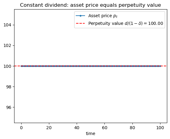
Max deviation from d/(1 - δ): 0.00e+00
For part b, substituting \(d_s = d\) and \(p_{T+1}^* = d/(1-\delta)\) into (11.7) gives
Exercise 11.7
For the growing dividend stream (\(d_{t+1} = 1.05 d_t\), \(d_0 = 1\), \(T = 6\), \(p_{T+1}^* = 10\)), plot the asset price at \(t = 0\) as a function of the discount factor \(\delta \in [0.90,\, 0.99]\).
Verify that \(p_0\) is strictly increasing in \(\delta\) and explain why in terms of the formula (11.7).
Solution to Exercise 11.7
T = 6
p_star = 10.0
d = np.array([1.0 * 1.05**t for t in range(T+1)])

δ_vals = np.linspace(0.90, 0.99, 200)
p0_vals = []

for δ in δ_vals:
    A = np.zeros((T+1, T+1))
    for i in range(T+1):
        A[i, i] = 1
        if i < T:
            A[i, i+1] = -δ
    b = np.zeros(T+1)
    b[-1] = δ * p_star
    p = np.linalg.solve(A, d + b)
    p0_vals.append(p[0])

fig, ax = plt.subplots()
ax.plot(δ_vals, p0_vals)
ax.set_xlabel(r'$\delta$')
ax.set_ylabel(r'$p_0$')
ax.set_title('Asset price at $t=0$ as a function of $\\delta$')
plt.show()
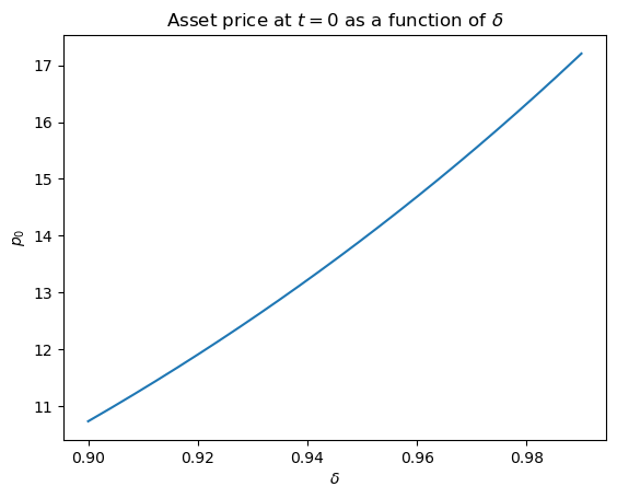
Each term \(\delta^{s-t} d_s\) in the fundamental component and the bubble term \(\delta^{T+1-t} p_{T+1}^*\) are both increasing in \(\delta\).
A higher discount factor therefore raises the present value of every future cash flow, pushing up \(p_0\).