33. Laffer Curves with Adaptive Expectations#
33.1. Overview#
This lecture studies stationary and dynamic Laffer curves in the inflation tax rate in a non-linear version of the model studied in this lecture Money Financed Government Deficits and Price Levels.
As in the lecture Money Financed Government Deficits and Price Levels, this lecture uses the log-linear version of the demand function for money that [Cagan, 1956] used in his classic paper in place of the linear demand function used in this lecture Money Financed Government Deficits and Price Levels.
But now, instead of assuming ‘‘rational expectations’’ in the form of ‘‘perfect foresight’’, we’ll adopt the ‘‘adaptive expectations’’ assumption used by [Cagan, 1956] and [Friedman, 1956].
This means that instead of assuming that expected inflation \(\pi_t^*\) is described by the “perfect foresight” or “rational expectations” hypothesis
that we adopted in lectures Money Financed Government Deficits and Price Levels and lectures Inflation Rate Laffer Curves, we’ll now assume that \(\pi_t^*\) is determined by the adaptive expectations hypothesis described in equation (33.4) reported below.
We shall discover that changing our hypothesis about expectations formation in this way will change some our findings and leave others intact. In particular, we shall discover that
replacing rational expectations with adaptive expectations leaves the two stationary inflation rates unchanged, but that \(\ldots\)
it reverses the perverse dynamics by making the lower stationary inflation rate the one to which the system typically converges
a more plausible comparative dynamic outcome emerges in which now inflation can be reduced by running lower government deficits
These more plausible comparative dynamics underlie the “old time religion” that states that “inflation is always and everywhere caused by government deficits”.
These issues were studied by [Bruno and Fischer, 1990].
Their purpose was to reverse what they thought were counter intuitive predictions of their model under rational expectations (i.e., perfect foresight in this context) by dropping rational expectations and instead assuming that people form expectations about future inflation rates according to the “adaptive expectations” scheme (33.4) described below.
Note
[Marcet and Sargent, 1989] had studied another way of selecting stationary equilibrium that involved replacing rational expectations with a model of learning via least squares regression.
[Marcet and Nicolini, 2003] and [Sargent et al., 2009] extended that work and applied it to study recurrent high-inflation episodes in Latin America.
33.2. The model#
Let
\(m_t\) be the log of the money supply at the beginning of time \(t\)
\(p_t\) be the log of the price level at time \(t\)
\(\pi_t^*\) be the public’s expectation of the rate of inflation between \(t\) and \(t+1\)
The law of motion of the money supply is
where \(g\) is the part of government expenditures financed by printing money.
Notice that equation (33.1) implies that
The demand function for money is
where \(\alpha \geq 0\).
Expectations of inflation are governed by
where \(\delta \in (0,1)\)
33.3. Computing an equilibrium sequence#
Equation the expressions for \(m_{t+1}\) provided by (33.3) and (33.2) and use equation (33.4) to eliminate \(\pi_t^*\) to obtain the following equation for \(p_t\):
Pseudo-code
Here is the pseudo-code for our algorithm.
Starting at time \(0\) with initial conditions \((m_0, \pi_{-1}^*, p_{-1})\), for each \(t \geq 0\) deploy the following steps in order:
solve (33.5) for \(p_t\)
solve equation (33.4) for \(\pi_t^*\)
solve equation (33.2) for \(m_{t+1}\)
This completes the algorithm.
33.4. Claims or conjectures#
It will turn out that
if they exist, limiting values \(\overline \pi\) and \(\overline \mu\) will be equal
if limiting values exist, there are two possible limiting values, one high, one low
unlike the outcome in lecture Inflation Rate Laffer Curves, for almost all initial log price levels and expected inflation rates \(p_0, \pi_{t}^*\), the limiting \(\overline \pi = \overline \mu\) is the lower steady state value
for each of the two possible limiting values \(\bar \pi\) ,there is a unique initial log price level \(p_0\) that implies that \(\pi_t = \mu_t = \bar \mu\) for all \(t \geq 0\)
this unique initial log price level solves \(\log(\exp(m_0) + g \exp(p_0)) - p_0 = - \alpha \bar \pi \)
the preceding equation for \(p_0\) comes from \(m_1 - p_0 = - \alpha \bar \pi\)
33.5. Limiting values of inflation rate#
As in our earlier lecture Inflation Rate Laffer Curves, we can compute the two prospective limiting values for \(\bar \pi\) by studying the steady-state Laffer curve.
Thus, in a steady state
where \(x > 0 \) is a common rate of growth of logarithms of the money supply and price level.
A few lines of algebra yields the following equation that \(x\) satisfies
where we require that
so that it is feasible to finance \(g\) by printing money.
The left side of (33.6) is steady state revenue raised by printing money.
The right side of (33.6) is the quantity of time \(t\) goods that the government raises by printing money.
Soon we’ll plot the left and right sides of equation (33.6).
But first we’ll write code that computes a steady-state \(\bar \pi\).
Let’s start by importing some libraries
from collections import namedtuple
import numpy as np
import matplotlib.pyplot as plt
from matplotlib.ticker import MaxNLocator
from matplotlib.cm import get_cmap
from matplotlib.colors import to_rgba
import matplotlib
from scipy.optimize import root, fsolve
Let’s create a namedtuple to store the parameters of the model
LafferAdaptive = namedtuple('LafferAdaptive',
                        ["m0",  # log of the money supply at t=0
                         "α",   # sensitivity of money demand
                         "g",   # government expenditure
                         "δ"])

# Create a Cagan Laffer model
def create_model(α=0.5, m0=np.log(100), g=0.35, δ=0.9):
    return LafferAdaptive(α=α, m0=m0, g=g, δ=δ)

model = create_model()
Now we write code that computes steady-state \(\bar \pi\)s.
# Define formula for π_bar
def solve_π(x, α, g):
    return np.exp(-α * x) - np.exp(-(1 + α) * x) - g

def solve_π_bar(model, x0):
    π_bar = fsolve(solve_π, x0=x0, xtol=1e-10, args=(model.α, model.g))[0]
    return π_bar

# Solve for the two steady state of π
π_l = solve_π_bar(model, x0=0.6)
π_u = solve_π_bar(model, x0=3.0)
print(f'The two steady state of π are: {π_l, π_u}')
The two steady state of π are: (np.float64(0.6737147075333034), np.float64(1.6930797322614815))
We find two steady state \(\bar \pi\) values
33.6. Steady-state Laffer curve#
The following figure plots the steady-state Laffer curve together with the two stationary inflation rates.
def compute_seign(x, α):
    return np.exp(-α * x) - np.exp(-(1 + α) * x)

def plot_laffer(model, πs):
    α, g = model.α, model.g

    # Generate π values
    x_values = np.linspace(0, 5, 1000)

    # Compute corresponding seigniorage values for the function
    y_values = compute_seign(x_values, α)

    # Plot the function
    plt.plot(x_values, y_values,
            label=f'$exp((-{α})x) - exp(- (1- {α}) x)$')
    for π, label in zip(πs, ['$\pi_l$', '$\pi_u$']):
        plt.text(π, plt.gca().get_ylim()[0]*2,
                 label, horizontalalignment='center',
                 color='brown', size=10)
        plt.axvline(π, color='brown', linestyle='--')
    plt.axhline(g, color='red', linewidth=0.5,
                linestyle='--', label='g')
    plt.xlabel('$\pi$')
    plt.ylabel('seigniorage')
    plt.legend()
    plt.show()

# Steady state Laffer curve
plot_laffer(model, (π_l, π_u))
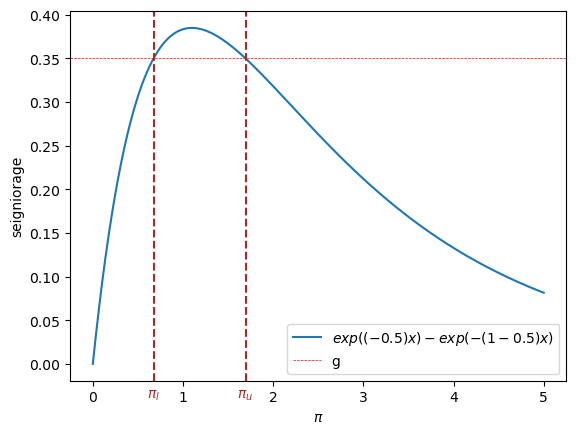
Fig. 33.1 Seigniorage as function of steady-state inflation. The dashed brown lines indicate \(\pi_l\) and \(\pi_u\).#
33.7. Associated initial price levels#
Now that we have our hands on the two possible steady states, we can compute two initial log price levels \(p_{-1}\), which as initial conditions, imply that \(\pi_t = \bar \pi \) for all \(t \geq 0\).
In particular, to initiate a fixed point of the dynamic Laffer curve dynamics, we set
def solve_p_init(model, π_star):
    m0, α = model.m0, model.α
    return m0 + α*π_star


# Compute two initial price levels associated with π_l and π_u
p_l, p_u = map(lambda π: solve_p_init(model, π), (π_l, π_u))
print('Associated initial p_{-1}s', f'are: {p_l, p_u}')
Associated initial p_{-1}s are: (np.float64(4.9420275397547435), np.float64(5.451710052118832))
33.7.1. Verification#
To start, let’s write some code to verify that if we initial \(\pi_{-1}^*,p_{-1}\) appropriately, the inflation rate \(\pi_t\) will be constant for all \(t \geq 0\) (at either \(\pi_u\) or \(\pi_l\) depending on the initial condition)
The following code verifies this.
def solve_laffer_adapt(p_init, π_init, model, num_steps):
    m0, α, δ, g = model.m0, model.α, model.δ, model.g

    m_seq = np.nan * np.ones(num_steps+1)
    π_seq = np.nan * np.ones(num_steps)
    p_seq = np.nan * np.ones(num_steps)
    μ_seq = np.nan * np.ones(num_steps)

    m_seq[1] = m0
    π_seq[0] = π_init
    p_seq[0] = p_init

    for t in range(1, num_steps):
        # Solve p_t
        def p_t(pt):
            return np.log(np.exp(m_seq[t]) + g * np.exp(pt)) \
                          - pt + α * ((1-δ)*(pt - p_seq[t-1]) + δ*π_seq[t-1])

        p_seq[t] = root(fun=p_t, x0=p_seq[t-1]).x[0]

        # Solve π_t
        π_seq[t] = (1-δ) * (p_seq[t]-p_seq[t-1]) + δ*π_seq[t-1]

        # Solve m_t
        m_seq[t+1] = np.log(np.exp(m_seq[t]) + g*np.exp(p_seq[t]))

        # Solve μ_t
        μ_seq[t] = m_seq[t+1] - m_seq[t]

    return π_seq, μ_seq, m_seq, p_seq
Compute limiting values starting from \(p_{-1}\) associated with \(\pi_l\)
π_seq, μ_seq, m_seq, p_seq = solve_laffer_adapt(p_l, π_l, model, 50)

# Check steady state m_{t+1} - m_t and p_{t+1} - p_t
print('m_{t+1} - m_t:', m_seq[-1] - m_seq[-2])
print('p_{t+1} - p_t:', p_seq[-1] - p_seq[-2])

# Check if exp(-αx) - exp(-(1 + α)x) = g
eq_g = lambda x: np.exp(-model.α * x) - np.exp(-(1 + model.α) * x)

print('eq_g == g:', np.isclose(eq_g(m_seq[-1] - m_seq[-2]), model.g))
m_{t+1} - m_t: 0.6737147075332999
p_{t+1} - p_t: 0.6737147075332928
eq_g == g: True
Compute limiting values starting from \(p_{-1}\) associated with \(\pi_u\)
π_seq, μ_seq, m_seq, p_seq = solve_laffer_adapt(p_u, π_u, model, 50)

# Check steady state m_{t+1} - m_t and p_{t+1} - p_t
print('m_{t+1} - m_t:', m_seq[-1] - m_seq[-2])
print('p_{t+1} - p_t:', p_seq[-1] - p_seq[-2])

# Check if exp(-αx) - exp(-(1 + α)x) = g
eq_g = lambda x: np.exp(-model.α * x) - np.exp(-(1 + model.α) * x)

print('eq_g == g:', np.isclose(eq_g(m_seq[-1] - m_seq[-2]), model.g))
m_{t+1} - m_t: 1.6930797322436035
p_{t+1} - p_t: 1.6930797322430209
eq_g == g: True
33.8. Slippery side of Laffer curve dynamics#
We are now equipped to compute time series starting from different \(p_{-1}, \pi_{-1}^*\) settings, analogous to those in this lecture Money Financed Government Deficits and Price Levels and this lecture Inflation Rate Laffer Curves.
Now we’ll study how outcomes unfold when we start \(p_{-1}, \pi_{-1}^*\) away from a stationary point of the dynamic Laffer curve, i.e., away from either \(\pi_u\) or \( \pi_l\).
To construct a perturbation pair \(\check p_{-1}, \check \pi_{-1}^*\)we’ll implement the following pseudo code:
set \(\check \pi_{-1}^* \) not equal to one of the stationary points \(\pi_u\) or \( \pi_l\).
set \(\check p_{-1} = m_0 + \alpha \check \pi_{-1}^*\)
Let’s simulate the result generated by varying the initial \(\pi_{-1}\) and corresponding \(p_{-1}\)
πs = np.linspace(π_l, π_u, 10)

line_params = {'lw': 1.5,
              'marker': 'o',
              'markersize': 3}

π_bars = (π_l, π_u)
draw_iterations(πs, model, line_params, π_bars, num_steps=80)
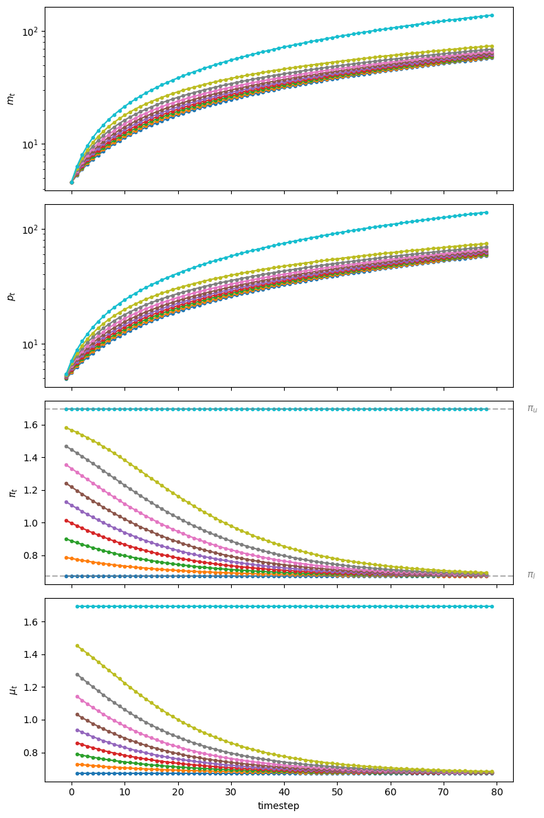
Fig. 33.2 Starting from different initial values of \(\pi_0\), paths of \(m_t\) (top panel, log scale for \(m\)), \(p_t\) (second panel, log scale for \(p\)), \(\pi_t\) (third panel), and \(\mu_t\) (bottom panel)#
33.9. Exercises#
Exercise 33.1
Comparative statics: how do steady-state inflation rates change with the government deficit \(g\)?
The lecture claims that, under adaptive expectations, the “old time religion” holds: lowering the government deficit \(g\) lowers the low-inflation steady state \(\pi_l\).
a. Compute the maximum seigniorage revenue \(g_{\rm max}\) and the corresponding
\(x_{\rm max}\) by finding the \(x\) that maximises \(\exp(-\alpha x) - \exp(-(1+\alpha)x)\)
using scipy.optimize.minimize_scalar.
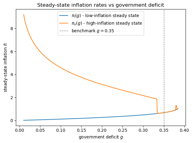
b. For \(g\) ranging from a small positive value to \(0.999 \times g_{\rm max}\), compute both \(\pi_l(g)\) and \(\pi_u(g)\) and plot them against \(g\) on the same axes.
c. Verify that the two roots merge as \(g \to g_{\rm max}\) and that \(\pi_l\) falls as \(g\) is reduced from the benchmark value \(g = 0.35\) to \(g/2\), then relate this to the “old time religion” claim in the lecture.
Solution
from scipy.optimize import minimize_scalar

# Part a: find g_max
res = minimize_scalar(lambda x: -compute_seign(x, model.α),
                      bounds=(0, 10), method='bounded')
x_max = res.x
g_max = compute_seign(x_max, model.α)
print(f"x_max  = {x_max:.4f}")
print(f"g_max  = {g_max:.4f}")
x_max  = 1.0986
g_max  = 0.3849
# Part b: trace π_l(g) and π_u(g)
g_grid  = np.linspace(0.01, g_max * 0.999, 300)
πl_list, πu_list = [], []

for g in g_grid:
    mod_g = create_model(g=g)
    πl_list.append(solve_π_bar(mod_g, x0=0.3))
    πu_list.append(solve_π_bar(mod_g, x0=4.0))

fig, ax = plt.subplots()
ax.plot(g_grid, πl_list, label=r'$\pi_l(g)$ - low-inflation steady state')
ax.plot(g_grid, πu_list, label=r'$\pi_u(g)$ - high-inflation steady state')
ax.axvline(model.g, color='grey', linestyle='--', lw=1,
           label=f'benchmark $g = {model.g}$')
ax.set_xlabel('government deficit $g$')
ax.set_ylabel('steady-state inflation $\\bar\\pi$')
ax.set_title('Steady-state inflation rates vs government deficit')
ax.legend()
plt.tight_layout()
plt.show()
# Part c: Verify "old time religion"
π_l_bench = solve_π_bar(model, x0=0.3)
π_l_half  = solve_π_bar(create_model(g=model.g / 2), x0=0.3)
print(f"π_l at g = {model.g:.2f}:      {π_l_bench:.4f}")
print(f"π_l at g = {model.g/2:.3f}:   {π_l_half:.4f}")
print(f"Cutting g in half reduces π_l by {π_l_bench - π_l_half:.4f}")
π_l at g = 0.35:      0.6737
π_l at g = 0.175:   0.2170
Cutting g in half reduces π_l by 0.4567
The two curves merge at \(g_{\rm max}\) because the Laffer curve peaks there and can no longer support two distinct inflation rates.
As \(g\) falls, \(\pi_l\) falls monotonically while \(\pi_u\) rises, confirming the “old time religion” that adaptive expectations select the low-inflation equilibrium where a lower deficit directly implies lower inflation.
Exercise 33.2
How the speed of expectation adjustment \(\delta\) affects convergence.
The parameter \(\delta \in (0,1)\) controls how slowly the public updates its inflation expectations: \(\delta\) close to \(1\) means expectations are very sluggish (heavily backward-looking), while \(\delta\) close to \(0\) means they adjust almost instantly.
Fix an initial \(\pi_0\) halfway between \(\pi_l\) and \(\pi_u\), i.e., \(\pi_0 = (\pi_l + \pi_u)/2\), and set \(p_{-1} = m_0 + \alpha \pi_0\).
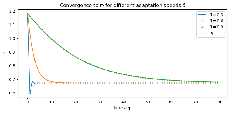
a. Using create_model and solve_laffer_adapt, simulate 80 steps for each
\(\delta \in \{0.3,\, 0.6,\, 0.9\}\), plot the resulting \(\pi_t\) paths on a
single panel, and add a horizontal dashed line at \(\pi_l\) for reference.
b. For each \(\delta\) value, report how many time steps it takes for \(\pi_t\) to come within \(0.01\) of \(\pi_l\).
c. Explain intuitively why a larger \(\delta\) leads to slower convergence.
Solution
δ_values  = [0.3, 0.6, 0.9]
num_steps = 80
π0 = (π_l + π_u) / 2          # start midway between the two steady states

fig, ax = plt.subplots(figsize=(8, 4))

for δ in δ_values:
    mod_δ = create_model(δ=δ)
    # Recompute steady states for this δ (they don't change, but confirm)
    π_l_δ = solve_π_bar(mod_δ, x0=0.6)
    p0    = mod_δ.m0 + mod_δ.α * π0
    π_seq, *_ = solve_laffer_adapt(p0, π0, mod_δ, num_steps)
    ax.plot(np.arange(num_steps), π_seq, lw=1.5, marker='o',
            markersize=2, label=f'$\\delta={δ}$')

ax.axhline(π_l, color='grey', linestyle='--', lw=1.5, alpha=0.7,
           label=r'$\pi_l$')
ax.set_xlabel('timestep')
ax.set_ylabel(r'$\pi_t$')
ax.set_title('Convergence to $\\pi_l$ for different adaptation speeds $\\delta$')
ax.legend()
plt.tight_layout()
plt.show()
# Part b: steps to come within 0.01 of π_l
tol = 0.01
print(f"{'δ':>5}  {'steps to |π_t - π_l| < 0.01':>30}")
print('-' * 40)
for δ in δ_values:
    mod_δ = create_model(δ=δ)
    p0    = mod_δ.m0 + mod_δ.α * π0
    π_seq, *_ = solve_laffer_adapt(p0, π0, mod_δ, num_steps)
    hits  = np.where(np.abs(π_seq - π_l) < tol)[0]
    steps = hits[0] if len(hits) > 0 else ">80"
    print(f"{δ:>5}  {str(steps):>30}")
    δ     steps to |π_t - π_l| < 0.01
----------------------------------------
  0.3                               3
  0.6                              10
  0.9                              72
Part c. When \(\delta\) is large, each period’s revision of \(\pi_t^*\) is a small fraction \((1-\delta)\) of the forecast error, so expectations are sticky.
This means the expectations signal that drives the economy toward \(\pi_l\) arrives only weakly each period, so the real inflation rate \(\pi_t\) creeps toward the steady state rather than jumping there quickly.
A small \(\delta\) gives forecast errors full or near-full weight, snapping expectations to the current observation and pulling \(\pi_t\) to \(\pi_l\) within just a few periods.