15. A Monetarist Theory of Price Levels#
15.1. Overview#
We’ll use linear algebra first to explain and then do some experiments with a “monetarist theory of price levels”.
Economists call it a “monetary” or “monetarist” theory of price levels because effects on price levels occur via a central bank’s decisions to print money supply.
a goverment’s fiscal policies determine whether its expenditures exceed its tax collections
if its expenditures exceed its tax collections, the government can instruct the central bank to cover the difference by printing money
that leads to effects on the price level as price level path adjusts to equate the supply of money to the demand for money
Such a theory of price levels was described by Thomas Sargent and Neil Wallace in chapter 5 of [Sargent, 2013], which reprints a 1981 Federal Reserve Bank of Minneapolis article entitled “Unpleasant Monetarist Arithmetic”.
Sometimes this theory is also called a “fiscal theory of price levels” to emphasize the importance of fiscal deficits in shaping changes in the money supply.
The theory has been extended, criticized, and applied by John Cochrane [Cochrane, 2023].
In another lecture price level histories, we described some European hyperinflations that occurred in the wake of World War I.
Elemental forces at work in the fiscal theory of the price level help to understand those episodes.
According to this theory, when the government persistently spends more than it collects in taxes and prints money to finance the shortfall (the “shortfall” is called the “government deficit”), it puts upward pressure on the price level and generates persistent inflation.
The “monetarist” or “fiscal theory of price levels” asserts that
to start a persistent inflation the government begins persistently to run a money-financed government deficit
to stop a persistent inflation the government stops persistently running a money-financed government deficit
The model in this lecture is a “rational expectations” (or “perfect foresight”) version of a model that Philip Cagan [Cagan, 1956] used to study the monetary dynamics of hyperinflations.
While Cagan didn’t use that “rational expectations” version of the model, Thomas Sargent [Sargent, 1982] did when he studied the Ends of Four Big Inflations in Europe after World War I.
this lecture fiscal theory of the price level with adaptive expectations describes a version of the model that does not impose “rational expectations” but instead uses what Cagan and his teacher Milton Friedman called “adaptive expectations”
a reader of both lectures will notice that the algebra is less complicated in the present rational expectations version of the model
the difference in algebra complications can be traced to the following source: the adaptive expectations version of the model has more endogenous variables and more free parameters
Some of our quantitative experiments with the rational expectations version of the model are designed to illustrate how the fiscal theory explains the abrupt end of those big inflations.
In those experiments, we’ll encounter an instance of a “velocity dividend” that has sometimes accompanied successful inflation stabilization programs.
To facilitate using linear matrix algebra as our main mathematical tool, we’ll use a finite horizon version of the model.
As in the present values and consumption smoothing lectures, our mathematical tools are matrix multiplication and matrix inversion.
15.2. Structure of the model#
The model consists of
a function that expresses the demand for real balances of government printed money as an inverse function of the public’s expected rate of inflation
an exogenous sequence of rates of growth of the money supply. The money supply grows because the government prints it to pay for goods and services
an equilibrium condition that equates the demand for money to the supply
a “perfect foresight” assumption that the public’s expected rate of inflation equals the actual rate of inflation.
To represent the model formally, let
\( m_t \) be the log of the supply of nominal money balances;
\(\mu_t = m_{t+1} - m_t \) be the net rate of growth of nominal balances;
\(p_t \) be the log of the price level;
\(\pi_t = p_{t+1} - p_t \) be the net rate of inflation between \(t\) and \( t+1\);
\(\pi_t^*\) be the public’s expected rate of inflation between \(t\) and \(t+1\);
\(T\) the horizon – i.e., the last period for which the model will determine \(p_t\)
\(\pi_{T+1}^*\) the terminal rate of inflation between times \(T\) and \(T+1\).
The demand for real balances \(\exp\left(m_t^d - p_t\right)\) is governed by the following version of the Cagan demand function
This equation asserts that the demand for real balances is inversely related to the public’s expected rate of inflation with sensitivity \(\alpha\).
People somehow acquire perfect foresight by their having solved a forecasting problem.
This lets us set
while equating demand for money to supply lets us set \(m_t^d = m_t\) for all \(t \geq 0\).
The preceding equations then imply
To fill in details about what it means for private agents to have perfect foresight, we subtract equation (15.3) at time \( t \) from the same equation at \( t+1\) to get
which we rewrite as a forward-looking first-order linear difference equation in \(\pi_s\) with \(\mu_s\) as a “forcing variable”:
where \( 0< \frac{\alpha}{1+\alpha} <1 \).
Setting \(\delta =\frac{\alpha}{1+\alpha}\), let’s us represent the preceding equation as
Write this system of \(T+1\) equations as the single matrix equation
By multiplying both sides of equation (15.4) by the inverse of the matrix on the left side, we can calculate
It turns out that
We can represent the equations
as the matrix equation
Multiplying both sides of equation (15.6) with the inverse of the matrix on the left will give
Equation (15.7) shows that the log of the money supply at \(t\) equals the log of the initial money supply \(m_0\) plus accumulation of rates of money growth between times \(0\) and \(T\).
15.3. Continuation values#
To determine the continuation inflation rate \(\pi_{T+1}^*\) we shall proceed by applying the following infinite-horizon version of equation (15.5) at time \(t = T+1\):
and by also assuming the following continuation path for \(\mu_t\) beyond \(T\):
Plugging the preceding equation into equation (15.8) at \(t = T+1\) and rearranging we can deduce that
where we require that \(\vert \gamma^* \delta \vert < 1\).
Let’s implement and solve this model.
As usual, we’ll start by importing some Python modules.
import numpy as np
from collections import namedtuple
import matplotlib.pyplot as plt
First, we store parameters in a namedtuple:
# Create the rational expectation version of Cagan model in finite time
CaganREE = namedtuple("CaganREE",
                        ["m0",    # initial money supply
                         "μ_seq", # sequence of rate of growth
                         "α",     # sensitivity parameter
                         "δ",     # α/(1 + α)
                         "π_end"  # terminal expected inflation
                        ])

def create_cagan_model(m0=1, α=5, μ_seq=None):
    δ = α/(1 + α)
    π_end = μ_seq[-1]    # compute terminal expected inflation
    return CaganREE(m0, μ_seq, α, δ, π_end)
Now we can solve the model to compute \(\pi_t\), \(m_t\) and \(p_t\) for \(t =1, \ldots, T+1\) using the matrix equation above
def solve(model, T):
    m0, π_end, μ_seq, α, δ = (model.m0, model.π_end,
                              model.μ_seq, model.α, model.δ)

    # Create matrix representation above
    A1 = np.eye(T+1, T+1) - δ * np.eye(T+1, T+1, k=1)
    A2 = np.eye(T+1, T+1) - np.eye(T+1, T+1, k=-1)

    # Assume γ* = 1
    b1 = (1-δ) * μ_seq + np.concatenate([np.zeros(T), [δ * π_end]])
    b2 = μ_seq + np.concatenate([[m0], np.zeros(T)])

    π_seq = np.linalg.solve(A1, b1)
    m_seq = np.linalg.solve(A2, b2)

    π_seq = np.append(π_seq, π_end)
    m_seq = np.append(m0, m_seq)

    p_seq = m_seq + α * π_seq

    return π_seq, m_seq, p_seq
15.3.1. Some quantitative experiments#
In the experiments below, we’ll use formula (15.9) as our terminal condition for expected inflation.
In devising these experiments, we’ll make assumptions about \(\{\mu_t\}\) that are consistent with formula (15.9).
We describe several such experiments.
In all of them,
so that, in terms of our notation and formula for \(\pi_{T+1}^*\) above, \(\gamma^* = 1\).
15.3.1.1. Experiment 1: Foreseen sudden stabilization#
In this experiment, we’ll study how, when \(\alpha >0\), a foreseen inflation stabilization has effects on inflation that proceed it.
We’ll study a situation in which the rate of growth of the money supply is \(\mu_0\) from \(t=0\) to \(t= T_1\) and then permanently falls to \(\mu^*\) at \(t=T_1\).
Thus, let \(T_1 \in (0, T)\).
So where \(\mu_0 > \mu^*\), we assume that
We’ll start by executing a version of our “experiment 1” in which the government implements a foreseen sudden permanent reduction in the rate of money creation at time \(T_1\).
Let’s experiment with the following parameters
T1 = 60
μ0 = 0.5
μ_star = 0
T = 80

μ_seq_1 = np.append(μ0*np.ones(T1), μ_star*np.ones(T-T1+1))

cm = create_cagan_model(μ_seq=μ_seq_1)

# solve the model
π_seq_1, m_seq_1, p_seq_1 = solve(cm, T)
Now we use the following function to plot the result
def plot_sequences(sequences, labels):
    fig, axs = plt.subplots(len(sequences), 1, figsize=(5, 12), dpi=200)
    for ax, seq, label in zip(axs, sequences, labels):
        ax.plot(range(len(seq)), seq, label=label)
        ax.set_ylabel(label)
        ax.set_xlabel('$t$')
        ax.legend()
    plt.tight_layout()
    plt.show()

sequences = (μ_seq_1, π_seq_1, m_seq_1 - p_seq_1, m_seq_1, p_seq_1)
plot_sequences(sequences, (r'$\mu$', r'$\pi$', r'$m - p$', r'$m$', r'$p$'))
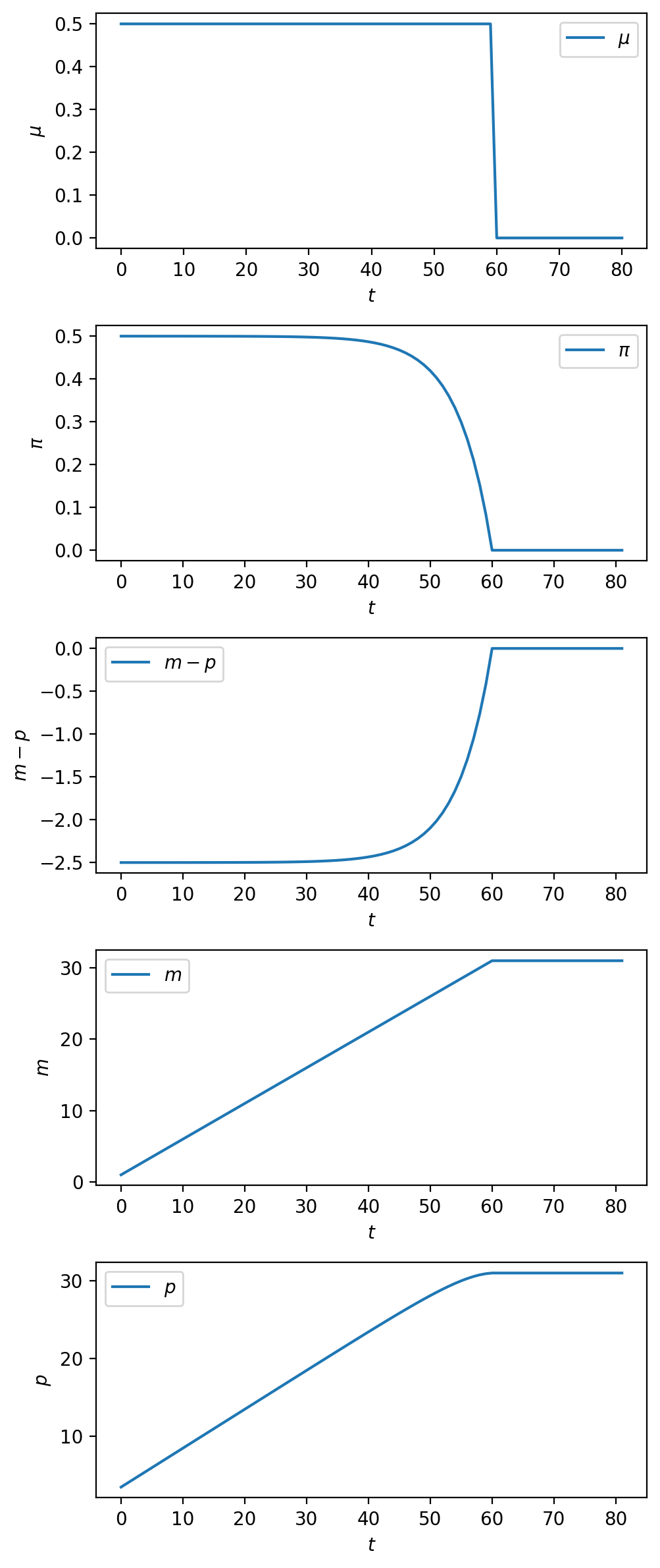
The plot of the money growth rate \(\mu_t\) in the top level panel portrays a sudden reduction from \(.5\) to \(0\) at time \(T_1 = 60\).
This brings about a gradual reduction of the inflation rate \(\pi_t\) that precedes the money supply growth rate reduction at time \(T_1\).
Notice how the inflation rate declines smoothly (i.e., continuously) to \(0\) at \(T_1\) – unlike the money growth rate, it does not suddenly “jump” downward at \(T_1\).
This is because the reduction in \(\mu\) at \(T_1\) has been foreseen from the start.
While the log money supply portrayed in the bottom panel has a kink at \(T_1\), the log price level does not – it is “smooth” – once again a consequence of the fact that the reduction in \(\mu\) has been foreseen.
To set the stage for our next experiment, we want to study the determinants of the price level a little more.
15.3.2. The log price level#
We can use equations (15.1) and (15.2) to discover that the log of the price level satisfies
or, by using equation (15.5),
In our next experiment, we’ll study a “surprise” permanent change in the money growth that beforehand was completely unanticipated.
At time \(T_1\) when the “surprise” money growth rate change occurs, to satisfy equation (15.10), the log of real balances jumps upward as \(\pi_t\) jumps downward.
But in order for \(m_t - p_t\) to jump, which variable jumps, \(m_{T_1}\) or \(p_{T_1}\)?
We’ll study that interesting question next.
15.3.3. What jumps?#
What jumps at \(T_1\)?
Is it \(p_{T_1}\) or \(m_{T_1}\)?
If we insist that the money supply \(m_{T_1}\) is locked at its value \(m_{T_1}^1\) inherited from the past, then formula (15.10) implies that the price level jumps downward at time \(T_1\), to coincide with the downward jump in \(\pi_{T_1}\)
An alternative assumption about the money supply level is that as part of the “inflation stabilization”, the government resets \(m_{T_1}\) according to
which describes how the government could reset the money supply at \(T_1\) in response to the jump in expected inflation associated with monetary stabilization.
Doing this would let the price level be continuous at \(T_1\).
By letting money jump according to equation (15.12) the monetary authority prevents the price level from falling at the moment that the unanticipated stabilization arrives.
In various research papers about stabilizations of high inflations, the jump in the money supply described by equation (15.12) has been called “the velocity dividend” that a government reaps from implementing a regime change that sustains a permanently lower inflation rate.
15.3.3.1. Technical details about whether \(p\) or \(m\) jumps at \(T_1\)#
We have noted that with a constant expected forward sequence \(\mu_s = \bar \mu\) for \(s\geq t\), \(\pi_{t} =\bar{\mu}\).
A consequence is that at \(T_1\), either \(m\) or \(p\) must “jump” at \(T_1\).
We’ll study both cases.
15.3.3.2. \(m_{T_{1}}\) does not jump.#
Simply glue the sequences \(t\leq T_1\) and \(t > T_1\).
15.3.3.3. \(m_{T_{1}}\) jumps.#
We reset \(m_{T_{1}}\) so that \(p_{T_{1}}=\left(m_{T_{1}-1}+\mu_{0}\right)+\alpha\mu_{0}\), with \(\pi_{T_{1}}=\mu^{*}\).
Then,
We then compute for the remaining \(T-T_{1}\) periods with \(\mu_{s}=\mu^{*},\forall s\geq T_{1}\) and the initial condition \(m_{T_{1}}\) from above.
We are now technically equipped to discuss our next experiment.
15.3.3.4. Experiment 2: an unforeseen sudden stabilization#
This experiment deviates a little bit from a pure version of our “perfect foresight” assumption by assuming that a sudden permanent reduction in \(\mu_t\) like that analyzed in experiment 1 is completely unanticipated.
Such a completely unanticipated shock is popularly known as an “MIT shock”.
The mental experiment involves switching at time \(T_1\) from an initial “continuation path” for \(\{\mu_t, \pi_t\} \) to another path that involves a permanently lower inflation rate.
Initial Path: \(\mu_t = \mu_0\) for all \(t \geq 0\).
This path is for \(\{\mu_t\}_{t=0}^\infty\); the associated path for \(\pi_t\) has \(\pi_t = \mu_0\).
Revised Continuation Path Where \( \mu_0 > \mu^*\), we construct a continuation path \(\{\mu_s\}_{s=T_1}^\infty\) by setting \(\mu_s = \mu^*\) for all \(s \geq T_1\). The perfect foresight continuation path for \(\pi\) is \(\pi_s = \mu^*\)
To capture a “completely unanticipated permanent shock to the \(\{\mu_t\}\) process at time \(T_1\), we simply glue the \(\mu_t, \pi_t\) that emerges under path 2 for \(t \geq T_1\) to the \(\mu_t, \pi_t\) path that had emerged under path 1 for \( t=0, \ldots, T_1 -1\).
We can do the MIT shock calculations mostly by hand.
Thus, for path 1, \(\pi_t = \mu_0 \) for all \(t \in [0, T_1-1]\), while for path 2, \(\mu_s = \mu^*\) for all \(s \geq T_1\).
We now move on to experiment 2, our “MIT shock”, completely unforeseen sudden stabilization.
We set this up so that the \(\{\mu_t\}\) sequences that describe the sudden stabilization are identical to those for experiment 1, the foreseen sudden stabilization.
The following code does the calculations and plots outcomes.
# path 1
μ_seq_2_path1 = μ0 * np.ones(T+1)

cm1 = create_cagan_model(μ_seq=μ_seq_2_path1)
π_seq_2_path1, m_seq_2_path1, p_seq_2_path1 = solve(cm1, T)

# continuation path
μ_seq_2_cont = μ_star * np.ones(T-T1+1)

cm2 = create_cagan_model(m0=m_seq_2_path1[T1],
                         μ_seq=μ_seq_2_cont)
π_seq_2_cont, m_seq_2_cont1, p_seq_2_cont1 = solve(cm2, T-T1)


# regime 1 - simply glue π_seq, μ_seq
μ_seq_2 = np.concatenate((μ_seq_2_path1[:T1],
                          μ_seq_2_cont))
π_seq_2 = np.concatenate((π_seq_2_path1[:T1],
                          π_seq_2_cont))
m_seq_2_regime1 = np.concatenate((m_seq_2_path1[:T1],
                                  m_seq_2_cont1))
p_seq_2_regime1 = np.concatenate((p_seq_2_path1[:T1],
                                  p_seq_2_cont1))

π_seq_2[T1-1] = p_seq_2_regime1[T1] - p_seq_2_regime1[T1-1]

# regime 2 - reset m_T1
m_T1 = (m_seq_2_path1[T1-1] + μ0) + cm2.α*(μ0 - μ_star)

cm3 = create_cagan_model(m0=m_T1, μ_seq=μ_seq_2_cont)
π_seq_2_cont2, m_seq_2_cont2, p_seq_2_cont2 = solve(cm3, T-T1)

m_seq_2_regime2 = np.concatenate((m_seq_2_path1[:T1],
                                  m_seq_2_cont2))
p_seq_2_regime2 = np.concatenate((p_seq_2_path1[:T1],
                                  p_seq_2_cont2))
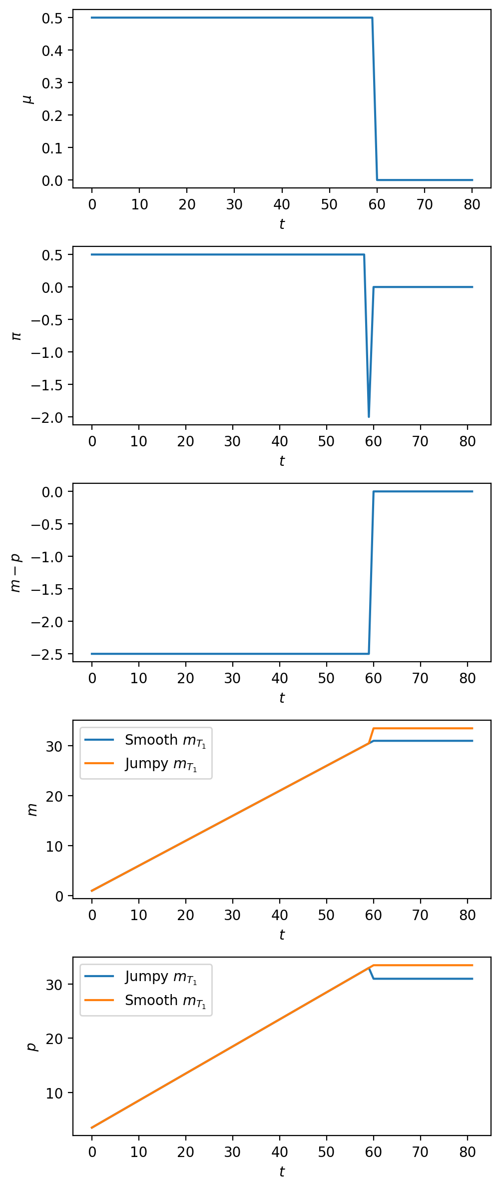
We invite you to compare these graphs with corresponding ones for the foreseen stabilization analyzed in experiment 1 above.
Note how the inflation graph in the second panel is now identical to the money growth graph in the top panel, and how now the log of real balances portrayed in the third panel jumps upward at time \(T_1\).
The bottom two panels plot \(m\) and \(p\) under two possible ways that \(m_{T_1}\) might adjust as required by the upward jump in \(m - p\) at \(T_1\).
the orange line lets \(m_{T_1}\) jump upward in order to make sure that the log price level \(p_{T_1}\) does not fall.
the blue line lets \(p_{T_1}\) fall while stopping the money supply from jumping.
Here is a way to interpret what the government is doing when the orange line policy is in place.
The government prints money to finance expenditure with the “velocity dividend” that it reaps from the increased demand for real balances brought about by the permanent decrease in the rate of growth of the money supply.
The next code generates a multi-panel graph that includes outcomes of both experiments 1 and 2.
That allows us to assess how important it is to understand whether the sudden permanent drop in \(\mu_t\) at \(t=T_1\) is fully anticipated, as in experiment 1, or completely unanticipated, as in experiment 2.
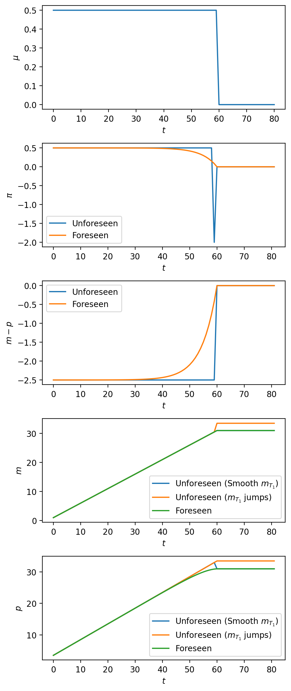
It is instructive to compare the preceding graphs with graphs of log price levels and inflation rates for data from four big inflations described in this lecture.
In particular, in the above graphs, notice how a gradual fall in inflation precedes the “sudden stop” when it has been anticipated long beforehand, but how inflation instead falls abruptly when the permanent drop in money supply growth is unanticipated.
It seems to the author team at quantecon that the drops in inflation near the ends of the four hyperinflations described in this lecture more closely resemble outcomes from the experiment 2 “unforeseen stabilization”.
(It is fair to say that the preceding informal pattern recognition exercise should be supplemented with a more formal structural statistical analysis.)
15.3.3.5. Experiment 3#
Foreseen gradual stabilization
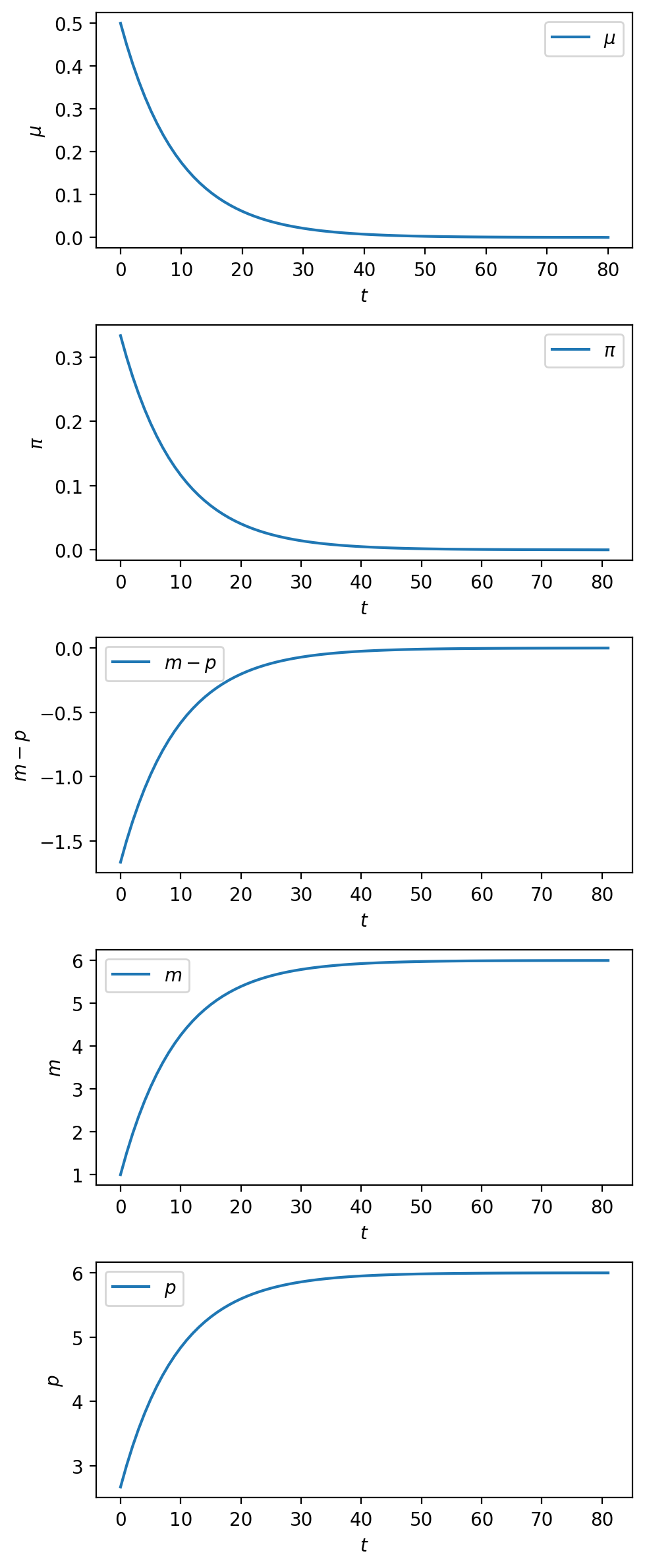
Instead of a foreseen sudden stabilization of the type studied with experiment 1, it is also interesting to study the consequences of a foreseen gradual stabilization.
Thus, suppose that \(\phi \in (0,1)\), that \(\mu_0 > \mu^*\), and that for \(t = 0, \ldots, T-1\)
Next we perform an experiment in which there is a perfectly foreseen gradual decrease in the rate of growth of the money supply.
The following code does the calculations and plots the results.
# parameters
ϕ = 0.9
μ_seq_stab = np.array([ϕ**t * μ0 + (1-ϕ**t)*μ_star for t in range(T)])
μ_seq_stab = np.append(μ_seq_stab, μ_star)

cm4 = create_cagan_model(μ_seq=μ_seq_stab)

π_seq_4, m_seq_4, p_seq_4 = solve(cm4, T)

sequences = (μ_seq_stab, π_seq_4,
             m_seq_4 - p_seq_4, m_seq_4, p_seq_4)
plot_sequences(sequences, (r'$\mu$', r'$\pi$',
                           r'$m - p$', r'$m$', r'$p$'))
15.4. Exercises#
Exercise 15.1
Sensitivity to \(\alpha\).
For Experiment 1 (foreseen sudden stabilization from \(\mu_0 = 0.5\) to \(\mu^* = 0\) at \(T_1 = 60\), with \(T = 80\)), solve the model for \(\alpha \in \{1,\, 3,\, 5,\, 10,\, 25\}\) and plot the inflation path \(\pi_t\) for each value on a single graph.
Describe how the anticipation effect, the pre-stabilization fall in inflation, changes with \(\alpha\).
Solution to Exercise 15.1
T1 = 60
μ0 = 0.5
μ_star = 0.0
T = 80
μ_seq = np.append(μ0 * np.ones(T1+1), μ_star * np.ones(T - T1))

α_vals = [1, 3, 5, 10, 25]
T_seq = np.arange(T+1)

fig, ax = plt.subplots()
for α in α_vals:
    cm = create_cagan_model(α=α, μ_seq=μ_seq)
    π_seq, _, _ = solve(cm, T)
    ax.plot(T_seq, π_seq[:-1], label=f'α = {α}')

ax.axvline(T1, linestyle='--', color='black', lw=1, label='Stabilization $T_1$')
ax.set_xlabel('$t$')
ax.set_ylabel(r'$\pi_t$')
ax.set_title('Inflation paths for different α (foreseen stabilization)')
ax.legend()
plt.show()
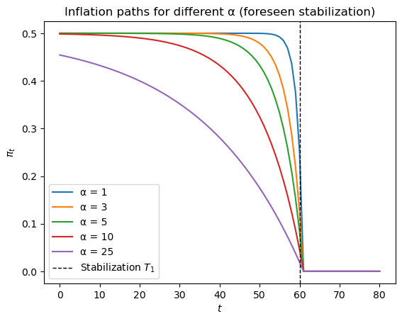
For small \(\alpha\), real-balance demand is insensitive to inflation, so the model behaves almost like the exogenous-money case and inflation tracks \(\mu_t\) closely.
For large \(\alpha\), agents strongly revalue money in response to expected future inflation, so the announcement of a future stabilization pulls inflation down gradually before \(T_1\).
Exercise 15.2
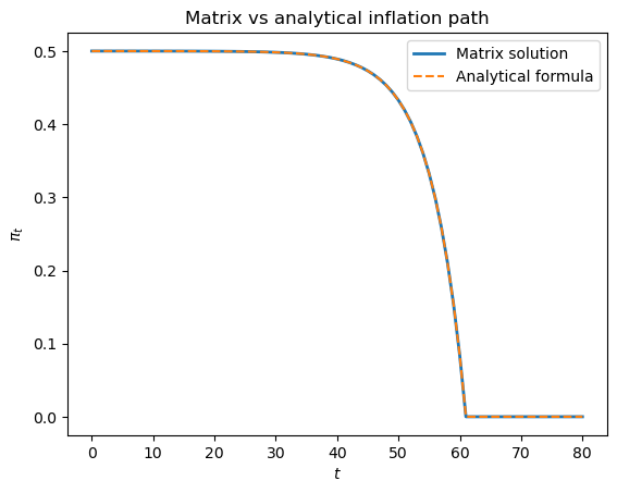
Verify the analytical formula.
For Experiment 1 (\(\alpha = 5\), \(T_1 = 60\), \(T = 80\), \(\mu_0 = 0.5\), \(\mu^* = 0\)), the closed-form solution for the inflation rate is given by equation (15.5):
Compute \(\pi_t\) directly from this formula for each \(t = 0, 1, \ldots, T\),
compare it to the matrix solution returned by solve, plot both on the same
graph, and print the maximum absolute difference.
Solution to Exercise 15.2
T1 = 60
μ0 = 0.5
μ_star = 0.0
T = 80
α = 5
μ_seq = np.append(μ0 * np.ones(T1+1), μ_star * np.ones(T - T1))

cm = create_cagan_model(α=α, μ_seq=μ_seq)
π_matrix, _, _ = solve(cm, T)
π_matrix = π_matrix[:-1]

δ = α / (1 + α)
π_term = cm.π_end
π_formula = np.array([
    (1 - δ) * sum(δ**(s-t) * μ_seq[s] for s in range(t, T+1))
    + δ**(T+1-t) * π_term
    for t in range(T+1)
])

T_seq = np.arange(T+1)
fig, ax = plt.subplots()
ax.plot(T_seq, π_matrix,  label='Matrix solution', lw=2)
ax.plot(T_seq, π_formula, '--', label='Analytical formula', lw=1.5)
ax.set_xlabel('$t$')
ax.set_ylabel(r'$\pi_t$')
ax.set_title('Matrix vs analytical inflation path')
ax.legend()
plt.show()

print(f'Max absolute difference: {np.max(np.abs(π_matrix - π_formula)):.2e}')
Max absolute difference: 2.78e-16
The two methods agree to machine precision, confirming that the matrix system (15.4) correctly implements formula (15.5).
Exercise 15.3
Foreseen gradual vs sudden stabilization.
Experiment 1 features a sudden foreseen drop in money growth at \(T_1 = 60\).
Experiment 3 features a gradual foreseen path \(\mu_t = \phi^t \mu_0 + (1-\phi^t)\mu^*\).
On a single graph, plot the inflation paths for:
Experiment 1 (sudden), and
Experiment 3 with \(\phi \in \{0.95, 0.85, 0.70\}\) (increasingly fast gradualism).
Use \(\alpha = 5\), \(\mu_0 = 0.5\), \(\mu^* = 0\), and \(T = 80\) to determine which approach generates the smoothest pre-stabilization decline in inflation.
Solution to Exercise 15.3
T = 80
T1 = 60
μ0 = 0.5
μ_star = 0.0
α = 5
T_seq = np.arange(T+1)

μ_sudden = np.append(μ0 * np.ones(T1+1), μ_star * np.ones(T - T1))
cm_sudden = create_cagan_model(α=α, μ_seq=μ_sudden)
π_sudden, _, _ = solve(cm_sudden, T)

fig, ax = plt.subplots()
ax.plot(T_seq, π_sudden[:-1], lw=2, label='Sudden (Exp. 1)')

for ϕ in [0.95, 0.85, 0.70]:
    μ_grad = np.array([ϕ**t * μ0 + (1 - ϕ**t) * μ_star for t in range(T)])
    μ_grad = np.append(μ_grad, μ_star)
    cm_grad = create_cagan_model(α=α, μ_seq=μ_grad)
    π_grad, _, _ = solve(cm_grad, T)
    ax.plot(T_seq, π_grad[:-1], label=f'Gradual ϕ = {ϕ}')

ax.set_xlabel('$t$')
ax.set_ylabel(r'$\pi_t$')
ax.set_title('Inflation: sudden vs gradual foreseen stabilization')
ax.legend()
plt.show()
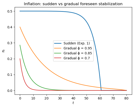
Faster gradual stabilization, corresponding to a smaller \(\phi\), pulls \(\mu_t\) down more quickly.
With less future inflation to discount, \(\pi_t\) falls sooner and more steeply.
The sudden stabilization has the largest discontinuity in the path of \(\mu_t\), but because it is fully anticipated the inflation path is smooth throughout.
Exercise 15.4
Real-balance dynamics.
For Experiments 1 and 2 (foreseen and unforeseen sudden stabilization, regime 1 where \(m_{T_1}\) is kept smooth), compute and plot the path of log real balances \(m_t - p_t\) for \(t = 0, 1, \ldots, T\).
Use \(\alpha = 5\), \(T_1 = 60\), \(T = 80\), \(\mu_0 = 0.5\), \(\mu^* = 0\).
Describe the qualitative difference between the two paths and explain it using the money-demand equation (15.1).
Solution to Exercise 15.4
T = 80
T1 = 60
μ0 = 0.5
μ_star = 0.0
α = 5

μ_seq_1 = np.append(μ0 * np.ones(T1+1), μ_star * np.ones(T - T1))
cm1 = create_cagan_model(α=α, μ_seq=μ_seq_1)
π_seq_1, m_seq_1, p_seq_1 = solve(cm1, T)

μ_seq_2a = μ0 * np.ones(T+1)
cm2a = create_cagan_model(α=α, μ_seq=μ_seq_2a)
π_pre, m_pre, p_pre = solve(cm2a, T)

μ_seq_2_cont = μ_star * np.ones(T-T1)
cm2b = create_cagan_model(m0=m_pre[T1+1], α=α,
                          μ_seq=μ_seq_2_cont)
π_post, m_post, p_post = solve(cm2b, T-1-T1)

m_unforeseen = np.concatenate((m_pre[:T1+1], m_post))
p_unforeseen = np.concatenate((p_pre[:T1+1], p_post))
T_seq = np.arange(T+1)

fig, ax = plt.subplots()
ax.plot(T_seq, (m_seq_1 - p_seq_1)[:-1], label='Foreseen (Exp. 1)')
ax.plot(T_seq, (m_unforeseen - p_unforeseen)[:-1],
        '--', label='Unforeseen (Exp. 2)')
ax.axvline(T1, linestyle=':', color='black', lw=1)
ax.set_xlabel('$t$')
ax.set_ylabel('$m_t - p_t$ (log real balances)')
ax.set_title('Real-balance paths: foreseen vs unforeseen stabilization')
ax.legend()
plt.show()
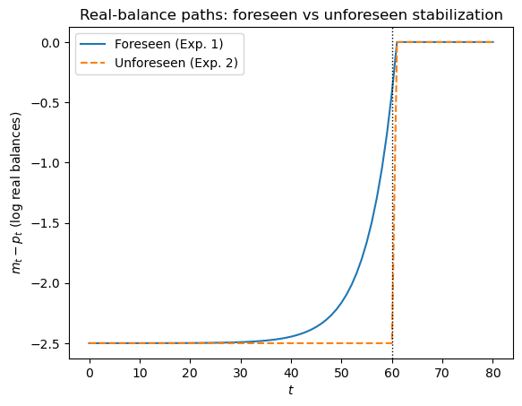
From equation (15.1), \(m_t - p_t = -\alpha \pi_t\).
In the foreseen case, inflation falls gradually before \(T_1\), so real balances rise smoothly as the public anticipates lower future inflation.
In the unforeseen case, there is no pre-announcement effect, so real balances are flat until the surprise at \(T_1\) and then jump upward with the drop in inflation.
15.5. Sequel#
Another lecture monetarist theory of price levels with adaptive expectations describes an “adaptive expectations” version of Cagan’s model.
The dynamics become more complicated and so does the algebra.
Nowadays, the “rational expectations” version of the model is more popular among central bankers and economists advising them.