25. The Solow-Swan Growth Model#
In this lecture we review a famous model due to Robert Solow (1925–2023) and Trevor Swan (1918–1989).
The model is used to study growth over the long run.
Although the model is simple, it contains some interesting lessons.
We will use the following imports.
import matplotlib.pyplot as plt
import numpy as np
25.1. The model#
In a Solow–Swan economy, agents save a fixed fraction of their current incomes.
Savings sustain or increase the stock of capital.
Capital is combined with labor to produce output, which in turn is paid out to workers and owners of capital.
To keep things simple, we ignore population and productivity growth.
For each integer \(t \geq 0\), output \(Y_t\) in period \(t\) is given by \(Y_t = F(K_t, L_t)\), where \(K_t\) is capital, \(L_t\) is labor and \(F\) is an aggregate production function.
The function \(F\) is assumed to be nonnegative and homogeneous of degree one, meaning that
Production functions with this property include
the Cobb-Douglas function \(F(K, L) = A K^{\alpha} L^{1-\alpha}\) with \(0 \leq \alpha \leq 1\).
the CES function \(F(K, L) = \left\{ a K^\rho + b L^\rho \right\}^{1/\rho}\) with \(a, b, \rho > 0\).
Here, \(\alpha\) is the output elasticity of capital and \(\rho\) is a parameter that determines the elasticity of substitution between capital and labor.
We assume a closed economy, so aggregate domestic investment equals aggregate domestic saving.
The saving rate is a constant \(s\) satisfying \(0 \leq s \leq 1\), so that aggregate investment and saving both equal \(s Y_t\).
Capital depreciates: without replenishing through investment, one unit of capital today becomes \(1-\delta\) units tomorrow.
Thus,
Without population growth, \(L_t\) equals some constant \(L\).
Setting \(k_t := K_t / L\) and using homogeneity of degree one now yields
With \(f(k) := F(k, 1)\), the final expression for capital dynamics is
Our aim is to learn about the evolution of \(k_t\) over time, given an exogenous initial capital stock \(k_0\).
25.2. A graphical perspective#
To understand the dynamics of the sequence \((k_t)_{t \geq 0}\) we use a 45-degree diagram.
To do so, we first need to specify the functional form for \(f\) and assign values to the parameters.
We choose the Cobb–Douglas specification \(f(k) = A k^\alpha\) and set \(A=2.0\), \(\alpha=0.3\), \(s=0.3\) and \(\delta=0.4\).
The function \(g\) from (25.1) is then plotted, along with the 45-degree line.
Let’s define the constants.
A, s, α, δ = 2, 0.3, 0.3, 0.4
x0 = 0.25
xmin, xmax = 0, 3
Now, we define the function \(g\).
def g(A, s, α, δ, k):
    return A * s * k**α + (1 - δ) * k
Let’s plot the 45-degree diagram of \(g\).
def plot45(kstar=None):
    xgrid = np.linspace(xmin, xmax, 12000)

    fig, ax = plt.subplots()

    ax.set_xlim(xmin, xmax)

    g_values = g(A, s, α, δ, xgrid)

    ymin, ymax = np.min(g_values), np.max(g_values)
    ax.set_ylim(ymin, ymax)

    lb = r'$g(k) = sAk^{\alpha} + (1 - \delta)k$'
    ax.plot(xgrid, g_values,  lw=2, alpha=0.6, label=lb)
    ax.plot(xgrid, xgrid, 'k-', lw=1, alpha=0.7, label=r'$45^{\circ}$')

    if kstar:
        fps = (kstar,)

        ax.plot(fps, fps, 'go', ms=10, alpha=0.6)

        ax.annotate(r'$k^* = (sA / \delta)^{(1/(1-\alpha))}$',
                 xy=(kstar, kstar),
                 xycoords='data',
                 xytext=(-40, -60),
                 textcoords='offset points',
                 fontsize=14,
                 arrowprops=dict(arrowstyle="->"))

    ax.legend(loc='upper left', frameon=False, fontsize=12)

    ax.set_xticks((0, 1, 2, 3))
    ax.set_yticks((0, 1, 2, 3))

    ax.set_xlabel('$k_t$', fontsize=12)
    ax.set_ylabel('$k_{t+1}$', fontsize=12)

    plt.show()
plot45()
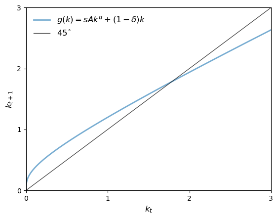
Suppose, at some \(k_t\), the value \(g(k_t)\) lies strictly above the 45-degree line.
Then we have \(k_{t+1} = g(k_t) > k_t\) and capital per worker rises.
If \(g(k_t) < k_t\) then capital per worker falls.
If \(g(k_t) = k_t\), then we are at a steady state and \(k_t\) remains constant.
(A steady state of the model is a fixed point of the mapping \(g\).)
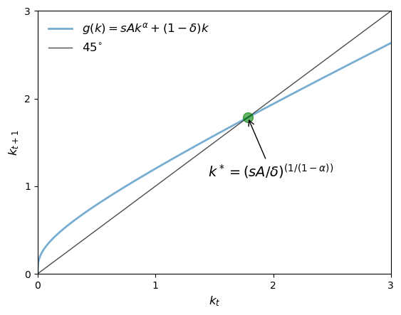
From the shape of the function \(g\) in the figure, we see that there is a unique steady state in \((0, \infty)\).
It solves \(k = s Ak^{\alpha} + (1-\delta)k\) and hence is given by
If initial capital is below \(k^*\), then capital increases over time.
If initial capital is above this level, then the reverse is true.
Let’s plot the 45-degree diagram to show the \(k^*\) in the plot.
kstar = ((s * A) / δ)**(1/(1 - α))
plot45(kstar)
From our graphical analysis, it appears that \((k_t)\) converges to \(k^*\), regardless of initial capital \(k_0\).
This is a form of global stability.
The next figure shows three time paths for capital, from three distinct initial conditions, under the parameterization listed above.
At this parameterization, \(k^* \approx 1.78\).
Let’s define the constants and three distinct initial conditions
A, s, α, δ = 2, 0.3, 0.3, 0.4
x0 = np.array([.25, 1.25, 3.25])

ts_length = 20
xmin, xmax = 0, ts_length
ymin, ymax = 0, 3.5
def simulate_ts(x0_values, ts_length):

    k_star = (s * A / δ)**(1/(1-α))
    fig, ax = plt.subplots(figsize=[11, 5])
    ax.set_xlim(xmin, xmax)
    ax.set_ylim(ymin, ymax)

    ts = np.zeros(ts_length)

    # simulate and plot time series
    for x_init in x0_values:
        ts[0] = x_init
        for t in range(1, ts_length):
            ts[t] = g(A, s, α, δ, ts[t-1])
        ax.plot(np.arange(ts_length), ts, '-o', ms=4, alpha=0.6,
                label=r'$k_0=%g$' %x_init)
    ax.plot(np.arange(ts_length), np.full(ts_length,k_star),
            alpha=0.6, color='red', label=r'$k^*$')
    ax.legend(fontsize=10)

    ax.set_xlabel(r'$t$', fontsize=14)
    ax.set_ylabel(r'$k_t$', fontsize=14)

    plt.show()
simulate_ts(x0, ts_length)
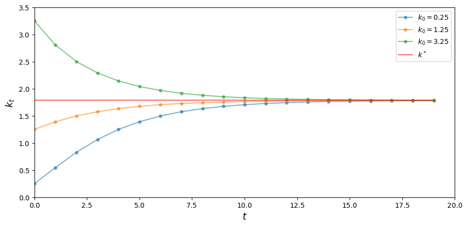
As expected, the time paths in the figure all converge to \(k^*\).
25.3. Growth in continuous time#
In this section, we investigate a continuous time version of the Solow–Swan growth model.
We will see how the smoothing provided by continuous time can simplify our analysis.
Recall that the discrete time dynamics for capital are given by \(k_{t+1} = s f(k_t) + (1 - \delta) k_t\).
A simple rearrangement gives the rate of change per unit of time:
Taking the time step to zero gives the continuous time limit
Our aim is to learn about the evolution of \(k_t\) over time, given an initial stock \(k_0\).
A steady state for (25.3) is a value \(k^*\) at which capital is unchanging, meaning \(k'_t = 0\) or, equivalently, \(s f(k^*) = \delta k^*\).
We assume \(f(k) = Ak^\alpha\), so \(k^*\) solves \(s A k^\alpha = \delta k\).
The solution is the same as the discrete time case—see (25.2).
The dynamics are represented in the next figure, maintaining the parameterization we used above.
Writing \(k'_t = g(k_t)\) with \(g(k) = s Ak^\alpha - \delta k\), values of \(k\) with \(g(k) > 0\) imply \(k'_t > 0\), so capital is increasing.
When \(g(k) < 0\), the opposite occurs. Once again, high marginal returns to savings at low levels of capital combined with low rates of return at high levels of capital combine to yield global stability.
To see this in a figure, let’s define the constants
A, s, α, δ = 2, 0.3, 0.3, 0.4
Next we define the function \(g\) for growth in continuous time
def g_con(A, s, α, δ, k):
    return A * s * k**α - δ * k
def plot_gcon(kstar=None):

    k_grid = np.linspace(0, 2.8, 10000)

    fig, ax = plt.subplots(figsize=[11, 5])
    ax.plot(k_grid, g_con(A, s, α, δ, k_grid), label='$g(k)$')
    ax.plot(k_grid, 0 * k_grid, label="$k'=0$")

    if kstar:
        fps = (kstar,)

        ax.plot(fps, 0, 'go', ms=10, alpha=0.6)


        ax.annotate(r'$k^* = (sA / \delta)^{(1/(1-\alpha))}$',
                 xy=(kstar, 0),
                 xycoords='data',
                 xytext=(0, 60),
                 textcoords='offset points',
                 fontsize=12,
                 arrowprops=dict(arrowstyle="->"))

    ax.legend(loc='lower left', fontsize=12)

    ax.set_xlabel("$k$",fontsize=10)
    ax.set_ylabel("$k'$", fontsize=10)

    ax.set_xticks((0, 1, 2, 3))
    ax.set_yticks((-0.3, 0, 0.3))

    plt.show()
kstar = ((s * A) / δ)**(1/(1 - α))
plot_gcon(kstar)
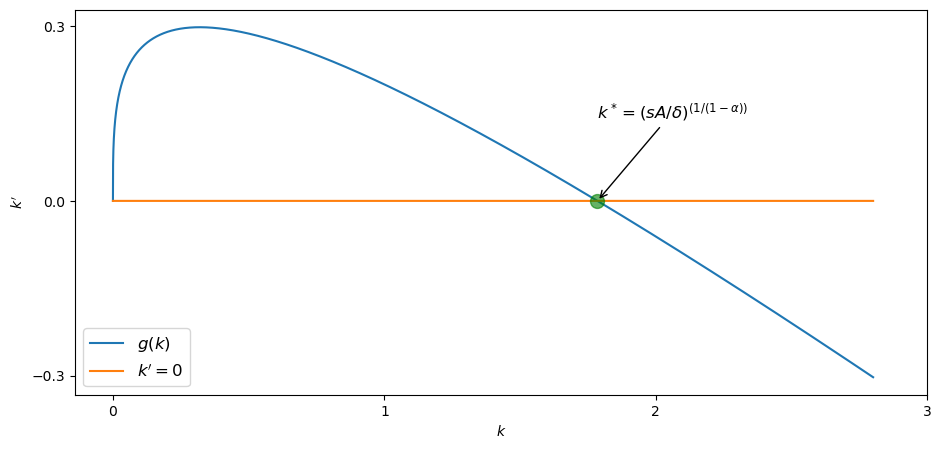
This shows global stability heuristically for a fixed parameterization, but how would we show the same thing formally for a continuum of plausible parameters?
In the discrete time case, a neat expression for \(k_t\) is hard to obtain.
In continuous time the process is easier: we can obtain a relatively simple expression for \(k_t\) that specifies the entire path.
The first step is to set \(x_t := k_t^{1-\alpha}\), so that \(x'_t = (1-\alpha) k_t^{-\alpha} k'_t\).
Substituting into \(k'_t = sAk_t^\alpha - \delta k_t\) leads to the linear differential equation
This equation, which is a linear ordinary differential equation, has the solution
(You can confirm that this function \(x_t\) satisfies (25.4) by differentiating it with respect to \(t\).)
Converting back to \(k_t\) yields
Since \(\delta > 0\) and \(\alpha \in (0, 1)\), we see immediately that \(k_t \to k^*\) as \(t \to \infty\) independent of \(k_0\).
Thus, global stability holds.
25.4. Exercises#
Exercise 25.1
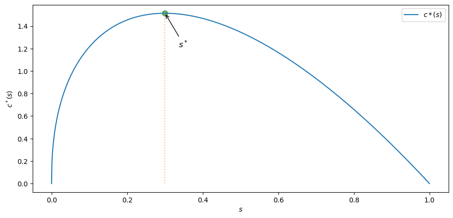
Plot per capita consumption \(c\) at the steady state, as a function of the savings rate \(s\), where \(0 \leq s \leq 1\).
Use the Cobb–Douglas specification \(f(k) = A k^\alpha\).
Set \(A=2.0, \alpha=0.3,\) and \(\delta=0.5\)
Also, find the approximate value of \(s\) that maximizes the \(c^*(s)\) and show it in the plot.
Solution to Exercise 25.1
Steady state consumption at savings rate \(s\) is given by
A = 2.0
α = 0.3
δ = 0.5
s_grid = np.linspace(0, 1, 1000)
k_star = ((s_grid * A) / δ)**(1/(1 - α))
c_star = (1 - s_grid) * A * k_star ** α
Let’s find the value of \(s\) that maximizes \(c^*\) using scipy.optimize.minimize_scalar.
We will use \(-c^*(s)\) since minimize_scalar finds the minimum value.
from scipy.optimize import minimize_scalar
def calc_c_star(s):
    k = ((s * A) / δ)**(1/(1 - α))
    return - (1 - s) * A * k ** α
return_values = minimize_scalar(calc_c_star, bounds=(0, 1))
s_star_max = return_values.x
c_star_max = -return_values.fun
print(f"Function is maximized at s = {round(s_star_max, 4)}")
Function is maximized at s = 0.3
x_s_max = np.array([s_star_max, s_star_max])
y_s_max = np.array([0, c_star_max])

fig, ax = plt.subplots(figsize=[11, 5])

fps = (c_star_max,)

# Highlight the maximum point with a marker
ax.plot((s_star_max, ), (c_star_max,), 'go', ms=8, alpha=0.6)

ax.annotate(r'$s^*$',
         xy=(s_star_max, c_star_max),
         xycoords='data',
         xytext=(20, -50),
         textcoords='offset points',
         fontsize=12,
         arrowprops=dict(arrowstyle="->"))
ax.plot(s_grid, c_star, label=r'$c*(s)$')
ax.plot(x_s_max, y_s_max, alpha=0.5, ls='dotted')
ax.set_xlabel(r'$s$')
ax.set_ylabel(r'$c^*(s)$')
ax.legend()

plt.show()
One can also try to solve this mathematically by differentiating \(c^*(s)\) and solve for \(\frac{d}{ds}c^*(s)=0\) using sympy.
from sympy import solve, Symbol, Rational
# Use Rational for exact symbolic computation
A = Rational(2)
α = Rational(3, 10)
δ = Rational(1, 2)

s_symbol = Symbol('s', real=True)
k = ((s_symbol * A) / δ)**(1/(1 - α))
c = (1 - s_symbol) * A * k ** α
Let’s differentiate \(c\) and solve using sympy.solve
# Solve using sympy
s_star = solve(c.diff())[0]
print(f"s_star = {float(s_star)}")
s_star = 0.3
Incidentally, the rate of savings which maximizes steady state level of per capita consumption is called the Golden Rule savings rate.
Exercise 25.2
Stochastic Productivity
To bring the Solow–Swan model closer to data, we need to think about handling random fluctuations in aggregate quantities.
Among other things, this will eliminate the unrealistic prediction that per-capita output \(y_t = A k^\alpha_t\) converges to a constant \(y^* := A (k^*)^\alpha\).
We shift to discrete time for the following discussion.
One approach is to replace constant productivity with some stochastic sequence \((A_t)_{t \geq 1}\).
Dynamics are now
We suppose \(f\) is Cobb–Douglas and \((A_t)\) is IID and lognormal.
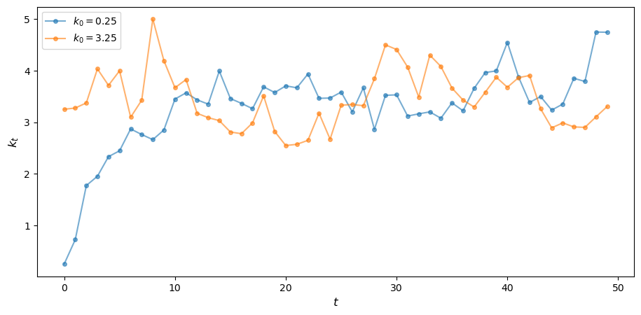
Now the long run convergence obtained in the deterministic case breaks down, since the system is hit with new shocks at each point in time.
Consider \(A=2.0, s=0.6, \alpha=0.3,\) and \(\delta=0.5\)
Generate and plot the time series \(k_t\).
Solution to Exercise 25.2
Let’s define the constants for lognormal distribution and initial values used for simulation
# Define the constants
σ = 0.2
μ = np.log(2) - σ**2 / 2
A = 2.0
s = 0.6
α = 0.3
δ = 0.5
x0 = [.25, 3.25] # list of initial values used for simulation
rng = np.random.default_rng()
Let’s define the function k_next to find the next value of \(k\)
def lgnorm():
    return np.exp(μ + σ * rng.standard_normal())

def k_next(s, α, δ, k):
    return lgnorm() * s * k**α + (1 - δ) * k
def ts_plot(x_values, ts_length):
    fig, ax = plt.subplots(figsize=[11, 5])
    ts = np.zeros(ts_length)

    # simulate and plot time series
    for x_init in x_values:
        ts[0] = x_init
        for t in range(1, ts_length):
            ts[t] = k_next(s, α, δ, ts[t-1])
        ax.plot(np.arange(ts_length), ts, '-o', ms=4,
                alpha=0.6, label=r'$k_0=%g$' %x_init)

    ax.legend(loc='best', fontsize=10)

    ax.set_xlabel(r'$t$', fontsize=12)
    ax.set_ylabel(r'$k_t$', fontsize=12)


    plt.show()
ts_plot(x0, 50)