16. Monetarist Theory of Price Levels with Adaptive Expectations#
16.1. Overview#
This lecture is a sequel or prequel to A Monetarist Theory of Price Levels.
We’ll use linear algebra to do some experiments with an alternative “monetarist” or “fiscal” theory of price levels.
Like the model in A Monetarist Theory of Price Levels, the model asserts that when a government persistently spends more than it collects in taxes and prints money to finance the shortfall, it puts upward pressure on the price level and generates persistent inflation.
Instead of the “perfect foresight” or “rational expectations” version of the model in A Monetarist Theory of Price Levels, our model in the present lecture is an “adaptive expectations” version of a model that [Cagan, 1956] used to study the monetary dynamics of hyperinflations.
It combines these components:
a demand function for real money balances that asserts that the logarithm of the quantity of real balances demanded depends inversely on the public’s expected rate of inflation
an adaptive expectations model that describes how the public’s anticipated rate of inflation responds to past values of actual inflation
an equilibrium condition that equates the demand for money to the supply
an exogenous sequence of rates of growth of the money supply
Our model stays quite close to Cagan’s original specification.
As in Present Values and Consumption Smoothing, the only linear algebra operations that we’ll be using are matrix multiplication and matrix inversion.
To facilitate using linear matrix algebra as our principal mathematical tool, we’ll use a finite horizon version of the model.
16.2. Structure of the model#
Let
\( m_t \) be the log of the supply of nominal money balances;
\(\mu_t = m_{t+1} - m_t \) be the net rate of growth of nominal balances;
\(p_t \) be the log of the price level;
\(\pi_t = p_{t+1} - p_t \) be the net rate of inflation between \(t\) and \( t+1\);
\(\pi_t^*\) be the public’s expected rate of inflation between \(t\) and \(t+1\);
\(T\) the horizon – i.e., the last period for which the model will determine \(p_t\)
\(\pi_0^*\) public’s initial expected rate of inflation between time \(0\) and time \(1\).
The demand for real balances \(\exp\left(m_t^d-p_t\right)\) is governed by the following version of the Cagan demand function
This equation asserts that the demand for real balances is inversely related to the public’s expected rate of inflation with sensitivity \(\alpha\).
Equating the logarithm \(m_t^d\) of the demand for money to the logarithm \(m_t\) of the supply of money in equation (16.1) and solving for the logarithm \(p_t\) of the price level gives
Taking the difference between equation (16.2) at time \(t+1\) and at time \(t\) gives
We assume that the expected rate of inflation \(\pi_t^*\) is governed by the following adaptive expectations scheme proposed by [Friedman, 1956] and [Cagan, 1956], where \(\lambda\in [0,1]\) denotes the weight on expected inflation.
As exogenous inputs into the model, we take initial conditions \(m_0, \pi_0^*\) and a money growth sequence \(\mu = \{\mu_t\}_{t=0}^T\).
As endogenous outputs of our model we want to find sequences \(\pi = \{\pi_t\}_{t=0}^T, p = \{p_t\}_{t=0}^T\) as functions of the exogenous inputs.
We’ll do some mental experiments by studying how the model outputs vary as we vary the model inputs.
16.3. Representing key equations with linear algebra#
We begin by writing the equation (16.4) adaptive expectations model for \(\pi_t^*\) for \(t=0, \ldots, T\) as
Write this equation as
where the \((T+2) \times (T+2) \)matrix \(A\), the \((T+2)\times (T+1)\) matrix \(B\), and the vectors \(\pi^* , \pi_0, \pi_0^*\) are defined implicitly by aligning these two equations.
Next we write the key equation (16.3) in matrix notation as
Represent the previous equation system in terms of vectors and matrices as
where the \((T+1) \times (T+2)\) matrix \(C\) is defined implicitly to align this equation with the preceding equation system.
16.4. Harvesting insights from our matrix formulation#
We now have all of the ingredients we need to solve for \(\pi\) as a function of \(\mu, \pi_0, \pi_0^*\).
Combine equations (16.5)and (16.6) to get
which implies that
Multiplying both sides of the above equation by the inverse of the matrix on the left side gives
Having solved equation (16.7) for \(\pi^*\), we can use equation (16.6) to solve for \(\pi\):
We have thus solved for two of the key endogenous time series determined by our model, namely, the sequence \(\pi^*\) of expected inflation rates and the sequence \(\pi\) of actual inflation rates.
Knowing these, we can then quickly calculate the associated sequence \(p\) of the logarithm of the price level from equation (16.2).
Let’s fill in the details for this step.
Since we now know \(\mu\) it is easy to compute \(m\).
Thus, notice that we can represent the equations
as the matrix equation
Multiplying both sides of equation (16.8) with the inverse of the matrix on the left will give
Equation (16.9) shows that the log of the money supply at \(t\) equals the log \(m_0\) of the initial money supply plus accumulation of rates of money growth between times \(0\) and \(t\).
We can then compute \(p_t\) for each \(t\) from equation (16.2).
We can write a compact formula for \(p \) as
where
which is just \(\pi^*\) with the last element dropped.
16.5. Forecast errors and model computation#
Our computations will verify that
so that in general
This outcome is typical in models in which adaptive expectations hypothesis like equation (16.4) appear as a component.
In A Monetarist Theory of Price Levels, we studied a version of the model that replaces hypothesis (16.4) with a “perfect foresight” or “rational expectations” hypothesis.
But now, let’s dive in and do some computations with the adaptive expectations version of the model.
As usual, we’ll start by importing some Python modules.
import numpy as np
from collections import namedtuple
import matplotlib.pyplot as plt
Cagan_Adaptive = namedtuple("Cagan_Adaptive",
                        ["α", "m0", "Eπ0", "T", "λ"])

def create_cagan_adaptive_model(α = 5, m0 = 1, Eπ0 = 0.5, T=80, λ = 0.9):
    return Cagan_Adaptive(α, m0, Eπ0, T, λ)

md = create_cagan_adaptive_model()
We solve the model and plot variables of interests using the following functions.
def solve_cagan_adaptive(model, μ_seq):
    " Solve the Cagan model in finite time. "
    α, m0, Eπ0, T, λ = model

    A = np.eye(T+2, T+2) - λ*np.eye(T+2, T+2, k=-1)
    B = np.eye(T+2, T+1, k=-1)
    C = -α*np.eye(T+1, T+2) + α*np.eye(T+1, T+2, k=1)
    Eπ0_seq = np.append(Eπ0, np.zeros(T+1))

    # Eπ_seq is of length T+2
    Eπ_seq = np.linalg.solve(A - (1-λ)*B @ C, (1-λ) * B @ μ_seq + Eπ0_seq)

    # π_seq is of length T+1
    π_seq = μ_seq + C @ Eπ_seq

    D = np.eye(T+1, T+1) - np.eye(T+1, T+1, k=-1) # D is the coefficient matrix in Equation (14.8)
    m0_seq = np.append(m0, np.zeros(T))

    # m_seq is of length T+2
    m_seq = np.linalg.solve(D, μ_seq + m0_seq)
    m_seq = np.append(m0, m_seq)

    # p_seq is of length T+2
    p_seq = m_seq + α * Eπ_seq

    return π_seq, Eπ_seq, m_seq, p_seq
def solve_and_plot(model, μ_seq):

    π_seq, Eπ_seq, m_seq, p_seq = solve_cagan_adaptive(model, μ_seq)

    T_seq = range(model.T+2)

    fig, ax = plt.subplots(5, 1, figsize=[5, 12], dpi=200)
    ax[0].plot(T_seq[:-1], μ_seq)
    ax[1].plot(T_seq[:-1], π_seq, label=r'$\pi_t$')
    ax[1].plot(T_seq, Eπ_seq, label=r'$\pi^{*}_{t}$')
    ax[2].plot(T_seq, m_seq - p_seq)
    ax[3].plot(T_seq, m_seq)
    ax[4].plot(T_seq, p_seq)

    y_labs = [r'$\mu$', r'$\pi$', r'$m - p$', r'$m$', r'$p$']
    subplot_title = [r'Money supply growth', r'Inflation', r'Real balances', r'Money supply', r'Price level']

    for i in range(5):
        ax[i].set_xlabel(r'$t$')
        ax[i].set_ylabel(y_labs[i])
        ax[i].set_title(subplot_title[i])

    ax[1].legend()
    plt.tight_layout()
    plt.show()

    return π_seq, Eπ_seq, m_seq, p_seq
16.6. Technical condition for stability#
In constructing our examples, we shall assume that \((\lambda, \alpha)\) satisfy
The source of this condition is the following string of deductions:
By assuring that the coefficient on \(\pi_t\) is less than one in absolute value, condition (16.11) assures stability of the dynamics of \(\{\pi_t\}\) described by the last line of our string of deductions.
The reader is free to study outcomes in examples that violate condition (16.11).
print(np.abs((md.λ - md.α*(1-md.λ))/(1 - md.α*(1-md.λ))))
0.8
16.7. Experiments#
Now we’ll turn to some experiments.
16.7.1. Experiment 1#
We’ll study a situation in which the rate of growth of the money supply is \(\mu_0\) from \(t=0\) to \(t= T_1\) and then permanently falls to \(\mu^*\) at \(t=T_1\).
Thus, let \(T_1 \in (0, T)\).
So where \(\mu_0 > \mu^*\), we assume that
Notice that we studied exactly this experiment in a rational expectations version of the model in A Monetarist Theory of Price Levels.
So by comparing outcomes across the two lectures, we can learn about consequences of assuming adaptive expectations, as we do here, instead of rational expectations as we assumed in that other lecture.
# Parameters for the experiment 1
T1 = 60
μ0 = 0.5
μ_star = 0

μ_seq_1 = np.append(μ0*np.ones(T1), μ_star*np.ones(md.T+1-T1))

# solve and plot
π_seq_1, Eπ_seq_1, m_seq_1, p_seq_1 = solve_and_plot(md, μ_seq_1)
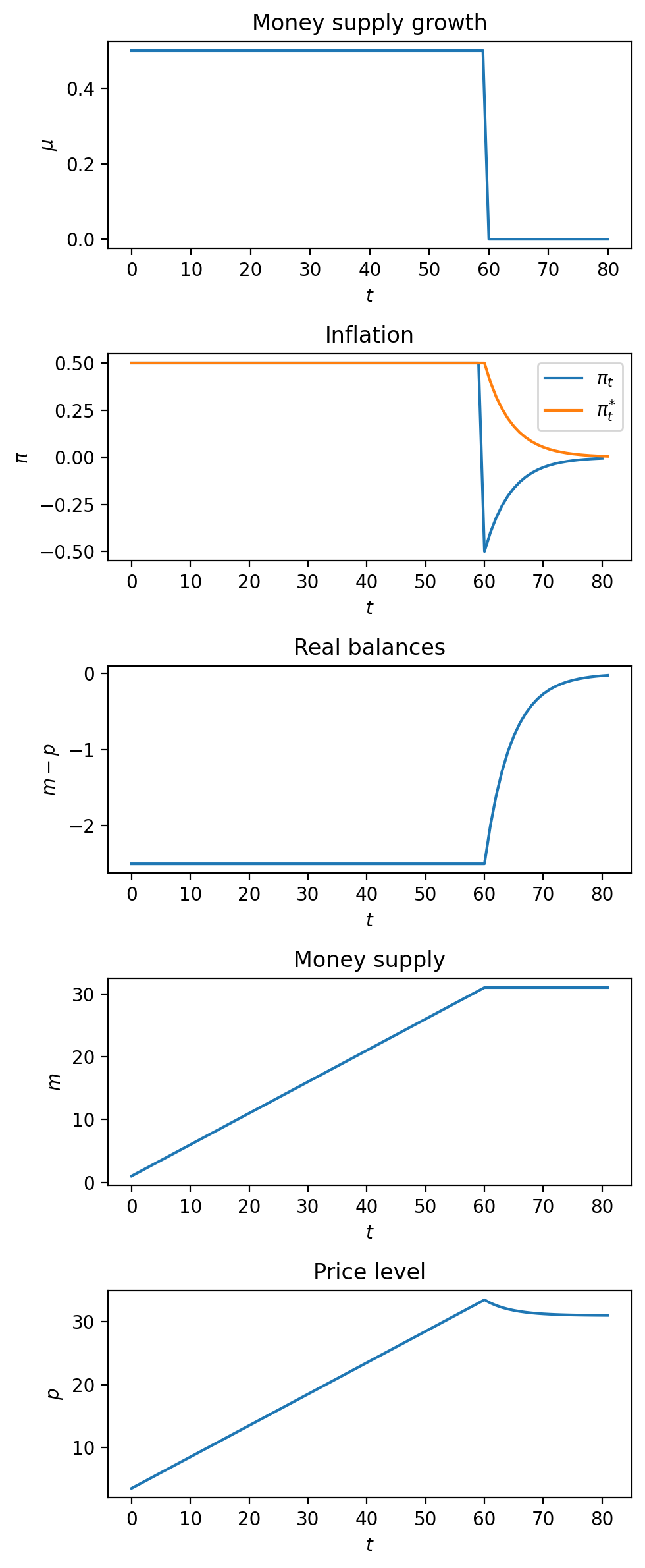
We invite the reader to compare outcomes with those under rational expectations studied in A Monetarist Theory of Price Levels.
Please note how the actual inflation rate \(\pi_t\) “overshoots” its ultimate steady-state value at the time of the sudden reduction in the rate of growth of the money supply at time \(T_1\).
We invite you to explain to yourself the source of this overshooting and why it does not occur in the rational expectations version of the model.
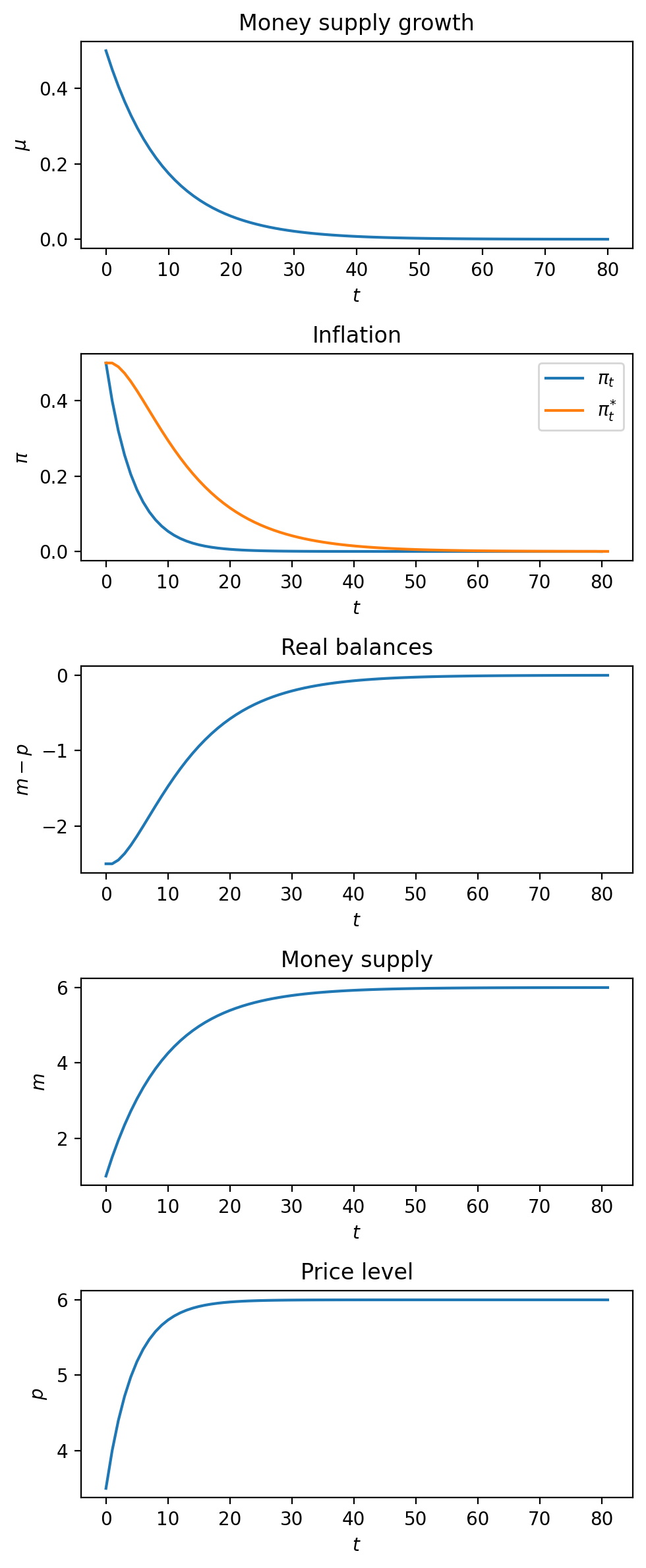
16.7.2. Experiment 2#
Now we’ll do a different experiment, namely, a gradual stabilization in which the rate of growth of the money supply smoothly declines from a high value to a persistently low value.
While price level inflation eventually falls, it falls more slowly than the driving force that ultimately causes it to fall, namely, the falling rate of growth of the money supply.
The sluggish fall in inflation is explained by how anticipated inflation \(\pi_t^*\) persistently exceeds actual inflation \(\pi_t\) during the transition from a high inflation to a low inflation situation.
# parameters
ϕ = 0.9
μ_seq_2 = np.array([ϕ**t * μ0 + (1-ϕ**t)*μ_star for t in range(md.T)])
μ_seq_2 = np.append(μ_seq_2, μ_star)


# solve and plot
π_seq_2, Eπ_seq_2, m_seq_2, p_seq_2 = solve_and_plot(md, μ_seq_2)
16.8. Exercises#
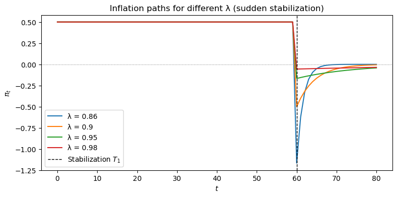
Exercise 16.1
Sensitivity of overshooting to the learning speed \(\lambda\).
For Experiment 1 (sudden stabilization at \(T_1 = 60\) from \(\mu_0 = 0.5\) to \(\mu^* = 0\)), solve the model for \(\lambda \in \{0.86,\, 0.90,\, 0.95,\, 0.98\}\) and, on a single graph, plot the actual inflation rate \(\pi_t\) for each value.
a. How do the sign and speed of post-stabilization convergence change as \(\lambda\) varies within the stable region?
b. For each \(\lambda\), print \(\rho\) and the peak absolute value of \(\pi_t\) for \(t \geq T_1\).
Solution to Exercise 16.1
T1 = 60
μ0 = 0.5
μ_star = 0.0
λ_vals = [0.86, 0.90, 0.95, 0.98]

fig, ax = plt.subplots(figsize=(9, 4))
for λ in λ_vals:
    m = create_cagan_adaptive_model(λ=λ)
    μ_seq = np.append(μ0 * np.ones(T1), μ_star * np.ones(m.T + 1 - T1))
    π_seq, _, _, _ = solve_cagan_adaptive(m, μ_seq)
    ax.plot(range(m.T + 1), π_seq, label=f'λ = {λ}')

ax.axvline(T1, linestyle='--', color='black', lw=1, label='Stabilization $T_1$')
ax.axhline(μ_star, linestyle=':', color='gray', lw=0.8)
ax.set_xlabel('$t$')
ax.set_ylabel(r'$\pi_t$')
ax.set_title('Inflation paths for different λ (sudden stabilization)')
ax.legend()
plt.show()

print(f'{"λ":>6} | {"ρ":>10} | {"|ρ|<1":>8} | {"peak |π| after T1":>20}')
print('-' * 56)
for λ in λ_vals:
    m = create_cagan_adaptive_model(λ=λ)
    μ_seq = np.append(μ0 * np.ones(T1), μ_star * np.ones(m.T + 1 - T1))
    π_seq, _, _, _ = solve_cagan_adaptive(m, μ_seq)
    ρ = (λ - m.α * (1 - λ)) / (1 - m.α * (1 - λ))
    peak = np.max(np.abs(π_seq[T1:]))
    print(f'{λ:>6.2f} | {ρ:>10.4f} | {str(abs(ρ) < 1):>8} | {peak:>20.4f}')
     λ |          ρ |    |ρ|<1 |    peak |π| after T1
--------------------------------------------------------
  0.86 |     0.5333 |     True |               1.1667
  0.90 |     0.8000 |     True |               0.5000
  0.95 |     0.9333 |     True |               0.1667
  0.98 |     0.9778 |     True |               0.0556
All four values satisfy the stability condition \(|\rho| < 1\) for the default \(\alpha = 5\) and have \(\rho > 0\).
The case \(\lambda = 0.86\) has the largest initial overshoot among these four values and then converges the fastest.
As \(\lambda\) moves closer to one, expectations become more inertial, so the post-stabilization response decays more slowly but starts from a smaller jump.
For \(\alpha = 5\), an oscillatory stable response would require \(0.8 < \lambda < 5/6\).
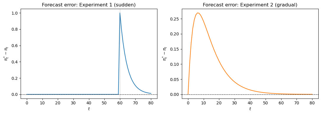
Exercise 16.2
Systematic forecast errors under adaptive expectations.
The lecture notes that \(\pi_t^* \neq \pi_t\) in general under adaptive expectations, in contrast to a rational-expectations equilibrium.
For the default model (md) and both experiments:
a. Compute and plot the forecast error \(e_t = \pi_t^* - \pi_t\) for \(t = 0, 1, \ldots, T\).
b. For each experiment, determine whether \(e_t\) is systematically positive or negative during the disinflation and explain why this systematic bias could not survive under rational expectations.
(Recall that Eπ_seq returned by solve_cagan_adaptive has \(T+2\) elements
while π_seq has \(T+1\); use Eπ_seq[:-1] to align them.)
Solution to Exercise 16.2
T1  = 60
μ0  = 0.5
μ_star = 0.0

# Experiment 1 sequences
μ_seq_1 = np.append(μ0 * np.ones(T1), μ_star * np.ones(md.T + 1 - T1))
π1, Eπ1, _, _ = solve_cagan_adaptive(md, μ_seq_1)

# Experiment 2 sequences
ϕ = 0.9
μ_seq_2 = np.array([ϕ**t * μ0 + (1 - ϕ**t) * μ_star for t in range(md.T)])
μ_seq_2 = np.append(μ_seq_2, μ_star)
π2, Eπ2, _, _ = solve_cagan_adaptive(md, μ_seq_2)

t_seq = np.arange(md.T + 1)
e1 = Eπ1[:-1] - π1   # forecast error, length T+1
e2 = Eπ2[:-1] - π2

fig, axes = plt.subplots(1, 2, figsize=(11, 4))
axes[0].plot(t_seq, e1)
axes[0].axhline(0, color='black', lw=0.8, linestyle='--')
axes[0].axvline(T1, color='gray', lw=0.8, linestyle=':')
axes[0].set_title('Forecast error: Experiment 1 (sudden)')
axes[0].set_xlabel('$t$')
axes[0].set_ylabel(r'$\pi_t^* - \pi_t$')

axes[1].plot(t_seq, e2, color='C1')
axes[1].axhline(0, color='black', lw=0.8, linestyle='--')
axes[1].set_title('Forecast error: Experiment 2 (gradual)')
axes[1].set_xlabel('$t$')
axes[1].set_ylabel(r'$\pi_t^* - \pi_t$')

plt.tight_layout()
plt.show()

print(f'Exp 1: mean forecast error t < T1:  {e1[:T1].mean():.4f}')
print(f'Exp 1: mean forecast error t >= T1: {e1[T1:].mean():.4f}')
print(f'Exp 2: mean forecast error overall: {e2.mean():.4f}')
Exp 1: mean forecast error t < T1:  0.0000
Exp 1: mean forecast error t >= T1: 0.2359
Exp 2: mean forecast error overall: 0.0617
During disinflation, actual inflation falls below expected inflation, so \(e_t = \pi_t^* - \pi_t > 0\) throughout the transition, so the public systematically over-predicts inflation.
Under rational expectations this persistent one-sided bias would be immediately arbitraged away as agents adjust their forecasting rule until \(e_t\) has mean zero.
Exercise 16.3
Post-stabilization convergence rate.
The lecture derives that, after the money-growth rate has been permanently set to \(\mu^*\), the actual inflation rate \(\pi_t\) decays geometrically:
Using Experiment 1 and the default model md:
a. Compute \(\rho\) analytically from the model parameters and verify that \(|\rho| < 1\) (the stability condition (16.11)).
b. From the solved path π_seq, compute the empirical ratios
\(\pi_{t+1}/\pi_t\) for \(t = T_1 + 1, \ldots, T_1 + 10\) and compare them
to \(\rho\).
c. Plot \(\log|\pi_t|\) against \(t\) for \(t \geq T_1\) and verify that it is linear with slope \(\log|\rho|\).
Solution to Exercise 16.3
T1 = 60
μ0 = 0.5
μ_star = 0.0

α, λ = md.α, md.λ
ρ = (λ - α * (1 - λ)) / (1 - α * (1 - λ))
print(f'α = {α},  λ = {λ}')
print(f'ρ = {ρ:.6f}   (|ρ| < 1: {abs(ρ) < 1})')

μ_seq = np.append(μ0 * np.ones(T1), μ_star * np.ones(md.T + 1 - T1))
π_seq, _, _, _ = solve_cagan_adaptive(md, μ_seq)

# Part b: empirical successive ratios
print(f'\n{"t":>5} | {"π_t":>12} | {"π_{t+1}/π_t":>14} | {"ρ":>8}')
print('-' * 46)
for t in range(T1, T1 + 10):
    ratio = π_seq[t + 1] / π_seq[t]
    print(f'{t:>5} | {π_seq[t]:>12.6f} | {ratio:>14.6f} | {ρ:>8.6f}')
α = 5,  λ = 0.9
ρ = 0.800000   (|ρ| < 1: True)

    t |          π_t |    π_{t+1}/π_t |        ρ
----------------------------------------------
   60 |    -0.500000 |       0.800000 | 0.800000
   61 |    -0.400000 |       0.800000 | 0.800000
   62 |    -0.320000 |       0.800000 | 0.800000
   63 |    -0.256000 |       0.800000 | 0.800000
   64 |    -0.204800 |       0.800000 | 0.800000
   65 |    -0.163840 |       0.800000 | 0.800000
   66 |    -0.131072 |       0.800000 | 0.800000
   67 |    -0.104858 |       0.800000 | 0.800000
   68 |    -0.083886 |       0.800000 | 0.800000
   69 |    -0.067109 |       0.800000 | 0.800000
# Part c: log|π_t| is linear after T1
t_post = np.arange(T1, md.T + 1)
log_π  = np.log(np.abs(π_seq[T1:]))

fig, ax = plt.subplots()
ax.plot(t_post, log_π, label=r'$\log|\pi_t|$')
# overlay the theoretical slope
slope_theory = np.log(abs(ρ))
ax.plot(t_post,
        log_π[0] + slope_theory * (t_post - T1),
        linestyle='--', label=f'slope = log|ρ| = {slope_theory:.4f}')
ax.set_xlabel('$t$')
ax.set_ylabel(r'$\log|\pi_t|$')
ax.set_title('Geometric decay of inflation after stabilization')
ax.legend()
plt.show()
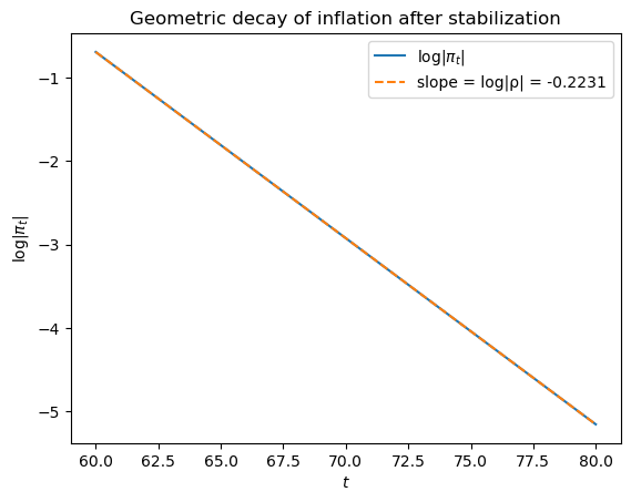
The empirical ratios converge to \(\rho = 0.8\) immediately after \(T_1\), confirming the first-order difference equation derived analytically.
The log plot is exactly linear with the theoretical slope, reflecting the exact geometric convergence \(\pi_t = \rho^{t-T_1} \pi_{T_1}\) for \(t \geq T_1\).
Exercise 16.4
Fast vs slow learning under gradual stabilization.
Experiment 2 uses a gradual decline in money growth \(\mu_t = \phi^t \mu_0 + (1-\phi^t)\mu^*\) with \(\phi = 0.9\).
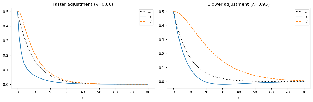
a. For the same gradual \(\mu\) path, compare the inflation \(\pi_t\) and expected inflation \(\pi_t^*\) paths for two stable cases:
* **Faster adjustment**: $\lambda = 0.86$
* **Slower adjustment**: $\lambda = 0.95$

Plot $\pi_t$, $\pi_t^*$, and $\mu_t$ for each case on side-by-side graphs.
b. For each case, compute the mean absolute forecast error \(\bar{e} = \frac{1}{T+1}\sum_{t=0}^T |\pi_t^* - \pi_t|\).
c. Explain why the faster-adjustment case can move below the money-growth path while the slower-adjustment case displays more persistent forecast errors.
Solution to Exercise 16.4
μ0    = 0.5
μ_star = 0.0
ϕ     = 0.9

λ_cases = {'Faster adjustment (λ=0.86)': 0.86,
           'Slower adjustment (λ=0.95)': 0.95}

fig, axes = plt.subplots(1, 2, figsize=(12, 4))

for ax, (label, λ) in zip(axes, λ_cases.items()):
    m = create_cagan_adaptive_model(λ=λ)
    μ_seq = np.array([ϕ**t * μ0 + (1 - ϕ**t) * μ_star for t in range(m.T)])
    μ_seq = np.append(μ_seq, μ_star)
    π_seq, Eπ_seq, _, _ = solve_cagan_adaptive(m, μ_seq)

    t_seq = np.arange(m.T + 1)
    ax.plot(t_seq, μ_seq,          label=r'$\mu_t$',   linestyle=':',  color='black')
    ax.plot(t_seq, π_seq,          label=r'$\pi_t$',   lw=1.5)
    ax.plot(t_seq, Eπ_seq[:-1],    label=r'$\pi_t^*$', linestyle='--', lw=1.5)
    ax.set_xlabel('$t$')
    ax.set_title(label)
    ax.legend(fontsize=8)

plt.tight_layout()
plt.show()

print(f'{"Case":>30} | {"Mean |forecast error|":>22}')
print('-' * 56)
for label, λ in λ_cases.items():
    m = create_cagan_adaptive_model(λ=λ)
    μ_seq = np.array([ϕ**t * μ0 + (1 - ϕ**t) * μ_star for t in range(m.T)])
    μ_seq = np.append(μ_seq, μ_star)
    π_seq, Eπ_seq, _, _ = solve_cagan_adaptive(m, μ_seq)
    mae = np.mean(np.abs(Eπ_seq[:-1] - π_seq))
    print(f'{label:>30} | {mae:>22.6f}')
                          Case |  Mean |forecast error|
--------------------------------------------------------
    Faster adjustment (λ=0.86) |               0.044085
    Slower adjustment (λ=0.95) |               0.122122
With faster adjustment, expectations revise downward more aggressively and inflation can move below the money-growth path during the transition.
With slower adjustment, expectations remain elevated for longer and the forecast errors are larger and slower to disappear.