30. Money Financed Government Deficits and Price Levels#
30.1. Overview#
This lecture extends and modifies the model in this lecture A Monetarist Theory of Price Levels by modifying the law of motion that governed the supply of money.
The model in this lecture consists of two components
a demand function for money
a law of motion for the supply of money
The demand function describes the public’s demand for “real balances”, defined as the ratio of nominal money balances to the price level
it assumes that the demand for real balance today varies inversely with the rate of inflation that the public forecasts to prevail between today and tomorrow
it assumes that the public’s forecast of that rate of inflation is perfect
The law of motion for the supply of money assumes that the government prints money to finance government expenditures
Our model equates the demand for money to the supply at each time \(t \geq 0\).
Equality between those demands and supply gives a dynamic model in which money supply and price level sequences are simultaneously determined by a set of simultaneous linear equations.
These equations take the form of what is often called vector linear difference equations.
In this lecture, we’ll roll up our sleeves and solve those equations in two different ways.
(One of the methods for solving vector linear difference equations will take advantage of a decomposition of a matrix that is studied in this lecture Eigenvalues and Eigenvectors.)
In this lecture we will encounter these concepts from macroeconomics:
an inflation tax that a government gathers by printing paper or electronic money
a dynamic Laffer curve in the inflation tax rate that has two stationary equilibria
perverse dynamics under rational expectations in which the system converges to the higher stationary inflation tax rate
a peculiar comparative stationary-state outcome connected with that stationary inflation rate: it asserts that inflation can be reduced by running higher government deficits, i.e., by raising more resources by printing money.
The same qualitative outcomes prevail in this lecture Inflation Rate Laffer Curves that studies a nonlinear version of the model in this lecture.
These outcomes set the stage for the analysis to be presented in this lecture Laffer Curves with Adaptive Expectations that studies a nonlinear version of the present model; it assumes a version of “adaptive expectations” instead of rational expectations.
That lecture will show that
replacing rational expectations with adaptive expectations leaves the two stationary inflation rates unchanged, but that \(\ldots\)
it reverses the perverse dynamics by making the lower stationary inflation rate the one to which the system typically converges
a more plausible comparative dynamic outcome emerges in which now inflation can be reduced by running lower government deficits
This outcome will be used to justify a selection of a stationary inflation rate that underlies the analysis of unpleasant monetarist arithmetic to be studied in this lecture Some Unpleasant Monetarist Arithmetic.
We’ll use these tools from linear algebra:
matrix multiplication
matrix inversion
eigenvalues and eigenvectors of a matrix
30.2. Demand for and supply of money#
We say demands and supplies (plurals) because there is one of each for each \(t \geq 0\).
Let
\(m_{t+1}\) be the supply of currency at the end of time \(t \geq 0\)
\(m_{t}\) be the supply of currency brought into time \(t\) from time \(t-1\)
\(g\) be the government deficit that is financed by printing currency at \(t \geq 1\)
\(m_{t+1}^d\) be the demand at time \(t\) for currency to bring into time \(t+1\)
\(p_t\) be the price level at time \(t\)
\(b_t = \frac{m_{t+1}}{p_t}\) is real balances at the end of time \(t\)
\(R_t = \frac{p_t}{p_{t+1}} \) be the gross rate of return on currency held from time \(t\) to time \(t+1\)
It is often helpful to state units in which quantities are measured:
\(m_t\) and \(m_t^d\) are measured in dollars
\(g\) is measured in time \(t\) goods
\(p_t\) is measured in dollars per time \(t\) goods
\(R_t\) is measured in time \(t+1\) goods per unit of time \(t\) goods
\(b_t\) is measured in time \(t\) goods
Our job now is to specify demand and supply functions for money.
We assume that the demand for currency satisfies the Cagan-like demand function
where \(\gamma_1, \gamma_2\) are positive parameters.
Now we turn to the supply of money.
We assume that \(m_0 >0\) is an “initial condition” determined outside the model.
We set \(m_0\) at some arbitrary positive value, say $100.
For \( t \geq 1\), we assume that the supply of money is determined by the government’s budget constraint
According to this equation, each period, the government prints money to pay for quantity \(g\) of goods.
In an equilibrium, the demand for currency equals the supply:
Let’s take a moment to think about what equation (30.3) tells us.
The demand for money at any time \(t\) depends on the price level at time \(t\) and the price level at time \(t+1\).
The supply of money at time \(t+1\) depends on the money supply at time \(t\) and the price level at time \(t\).
So the infinite sequence of equations (30.3) for \( t \geq 0\) imply that the sequences \(\{p_t\}_{t=0}^\infty\) and \(\{m_t\}_{t=0}^\infty\) are tied together and ultimately simulataneously determined.
30.3. Equilibrium price and money supply sequences#
The preceding specifications imply that for \(t \geq 1\), real balances evolve according to
or
The demand for real balances is
We’ll restrict our attention to parameter values and associated gross real rates of return on real balances that assure that the demand for real balances is positive, which according to (30.5) means that
which implies that
Gross real rate of return \(\underline R\) is the smallest rate of return on currency that is consistent with a nonnegative demand for real balances.
We shall describe two distinct but closely related ways of computing a pair \(\{p_t, m_t\}_{t=0}^\infty\) of sequences for the price level and money supply.
But first it is instructive to describe a special type of equilibrium known as a steady state.
In a steady-state equilibrium, a subset of key variables remain constant or invariant over time, while remaining variables can be expressed as functions of those constant variables.
Finding such state variables is something of an art.
In many models, a good source of candidates for such invariant variables is a set of ratios.
This is true in the present model.
30.3.1. Steady states#
In a steady-state equilibrium of the model we are studying,
for \(t \geq 0\).
Notice that both \(R_t = \frac{p_t}{p_{t+1}}\) and \(b_t = \frac{m_{t+1}}{p_t} \) are ratios.
To compute a steady state, we seek gross rates of return on currency and real balances \(\bar R, \bar b\) that satisfy steady-state versions of both the government budget constraint and the demand function for real balances:
Together these equations imply
The left side is the steady-state amount of seigniorage or government revenues that the government gathers by paying a gross rate of return \(\bar R \le 1\) on currency.
The right side is government expenditures.
Define steady-state seigniorage as
Notice that \(S(\bar R) \geq 0\) only when \(\bar R \in [\frac{\gamma_2}{\gamma_1}, 1] \equiv [\underline R, \overline R]\) and that \(S(\bar R) = 0\) if \(\bar R = \underline R\) or if \(\bar R = \overline R\).
We shall study equilibrium sequences that satisfy
Maximizing steady-state seigniorage (30.8) with respect to \(\bar R\), we find that the maximizing rate of return on currency is
and that the associated maximum seigniorage revenue that the government can gather from printing money is
It is useful to rewrite equation (30.7) as
A steady state gross rate of return \(\bar R\) solves quadratic equation (30.9).
So two steady states typically exist.
30.4. Some code#
Let’s start with some imports:
import numpy as np
import matplotlib.pyplot as plt
from matplotlib.ticker import MaxNLocator
plt.rcParams['figure.dpi'] = 300
from collections import namedtuple
Let’s set some parameter values and compute possible steady-state rates of return on currency \(\bar R\), the seigniorage maximizing rate of return on currency, and an object that we’ll discuss later, namely, an initial price level \(p_0\) associated with the maximum steady-state rate of return on currency.
First, we create a namedtuple to store parameters so that we can reuse this namedtuple in our functions throughout this lecture
# Create a namedtuple that contains parameters
MoneySupplyModel = namedtuple("MoneySupplyModel",
                        ["γ1", "γ2", "g",
                         "M0", "R_u", "R_l"])

def create_model(γ1=100, γ2=50, g=3.0, M0=100):

    # Calculate the steady states for R
    R_steady = np.roots((-γ1, γ1 + γ2 - g, -γ2))
    R_u, R_l = R_steady
    print("[R_u, R_l] =", R_steady)

    return MoneySupplyModel(γ1=γ1, γ2=γ2, g=g, M0=M0, R_u=R_u, R_l=R_l)
Now we compute the \(\bar R_{\rm max}\) and corresponding revenue
def seign(R, model):
    γ1, γ2, g = model.γ1, model.γ2, model.g
    return -γ2/R + (γ1 + γ2)  - γ1 * R

msm = create_model()

# Calculate initial guess for p0
p0_guess = msm.M0 / (msm.γ1 - msm.g - msm.γ2 / msm.R_u)
print(f'p0 guess = {p0_guess:.4f}')

# Calculate seigniorage maximizing rate of return
R_max = np.sqrt(msm.γ2/msm.γ1)
g_max = seign(R_max, msm)
print(f'R_max, g_max = {R_max:.4f}, {g_max:.4f}')
[R_u, R_l] = [0.93556171 0.53443829]
p0 guess = 2.2959
R_max, g_max = 0.7071, 8.5786
Now let’s plot seigniorage as a function of alternative potential steady-state values of \(R\).
We’ll see that there are two steady-state values of \(R\) that attain seigniorage levels equal to \(g\), one that we’ll denote \(R_\ell\), another that we’ll denote \(R_u\).
They satisfy \(R_\ell < R_u\) and are affiliated with a higher inflation tax rate \((1-R_\ell)\) and a lower inflation tax rate \(1 - R_u\).
# Generate values for R
R_values = np.linspace(msm.γ2/msm.γ1, 1, 250)

# Calculate the function values
seign_values = seign(R_values, msm)

# Visualize seign_values against R values
fig, ax = plt.subplots(figsize=(11, 5))
plt.plot(R_values, seign_values, label='inflation tax revenue')
plt.axhline(y=msm.g, color='red', linestyle='--', label='government deficit')
plt.xlabel('$R$')
plt.ylabel('seigniorage')

plt.legend()
plt.show()
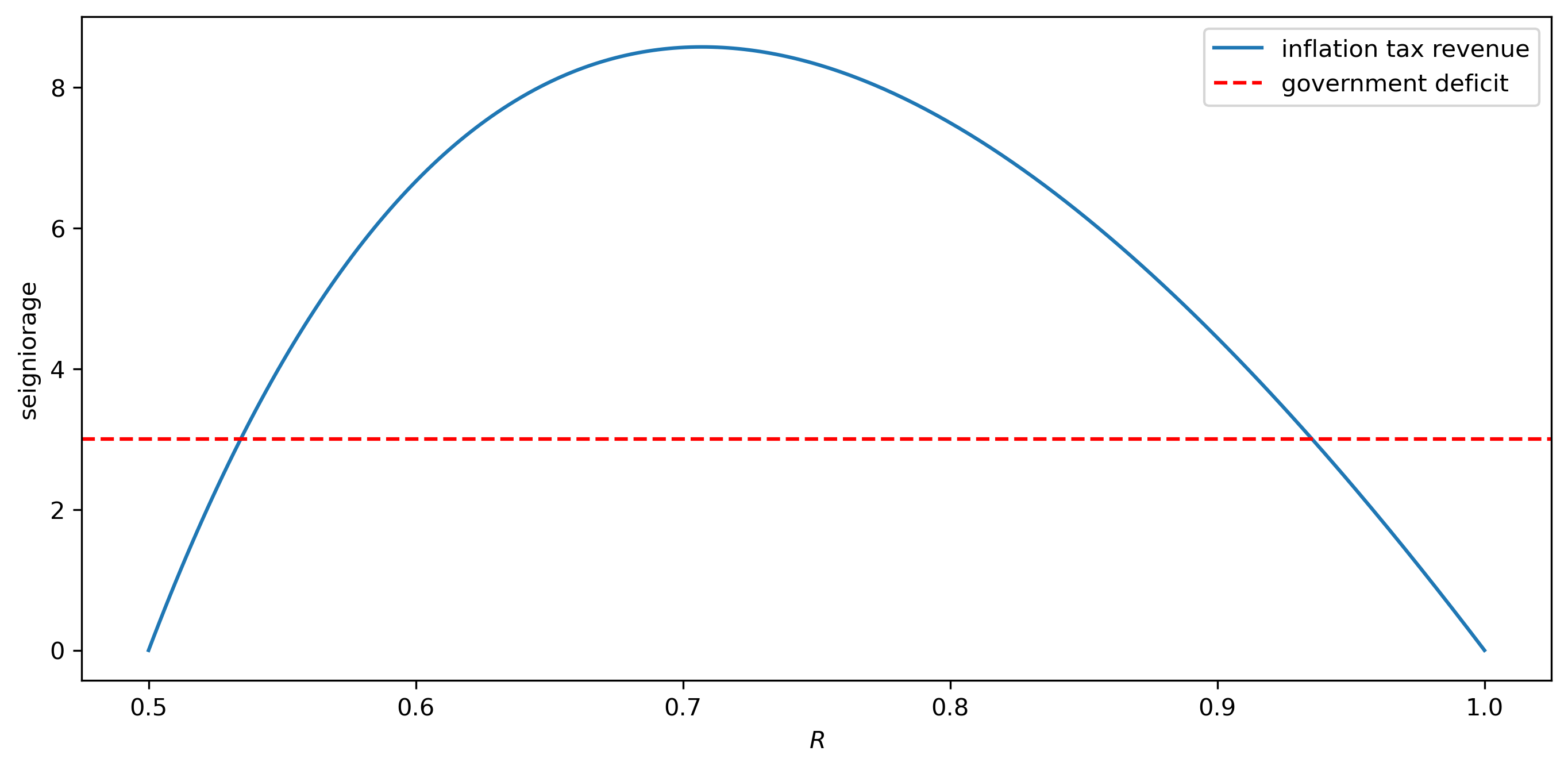
Fig. 30.1 Steady state revenue from inflation tax as function of steady state gross return on currency (solid blue curve) and real government expenditures (dotted red line) plotted against steady-state rate of return currency#
Let’s print the two steady-state rates of return \(\bar R\) and the associated seigniorage revenues that the government collects.
(By construction, both steady-state rates of return should raise the same amounts real revenue.)
We hope that the following code will confirm this.
g1 = seign(msm.R_u, msm)
print(f'R_u, g_u = {msm.R_u:.4f}, {g1:.4f}')

g2 = seign(msm.R_l, msm)
print(f'R_l, g_l = {msm.R_l:.4f}, {g2:.4f}')
R_u, g_u = 0.9356, 3.0000
R_l, g_l = 0.5344, 3.0000
Now let’s compute the maximum steady-state amount of seigniorage that could be gathered by printing money and the state-state rate of return on money that attains it.
30.5. Two computation strategies#
We now proceed to compute equilibria, not necessarily steady states.
We shall deploy two distinct computation strategies.
30.5.1. Method 1#
set \(R_0 \in [\frac{\gamma_2}{\gamma_1}, R_u]\) and compute \(b_0 = \gamma_1 - \gamma_2/R_0\).
compute sequences \(\{R_t, b_t\}_{t=1}^\infty\) of rates of return and real balances that are associated with an equilibrium by solving equation (30.4) and (30.5) sequentially for \(t \geq 1\):
Construct the associated equilibrium \(p_0\) from
compute \(\{p_t, m_t\}_{t=1}^\infty\) by solving the following equations sequentially
Remark 30.1
Method 1 uses an indirect approach to computing an equilibrium by first computing an equilibrium \(\{R_t, b_t\}_{t=0}^\infty\) sequence and then using it to back out an equilibrium \(\{p_t, m_t\}_{t=0}^\infty\) sequence.
Remark 30.2
Notice that method 1 starts by picking an initial condition \(R_0\) from a set \([\frac{\gamma_2}{\gamma_1}, R_u]\).
Equilibrium \(\{p_t, m_t\}_{t=0}^\infty\) sequences are not unique.
There is actually a continuum of equilibria indexed by a choice of \(R_0\) from the set \([\frac{\gamma_2}{\gamma_1}, R_u]\).
Remark 30.3
Associated with each selection of \(R_0\) there is a unique \(p_0\) described by equation (30.11).
30.5.2. Method 2#
This method deploys a direct approach. It defines a “state vector” \(y_t = \begin{bmatrix} m_t \cr p_t\end{bmatrix} \) and formulates equilibrium conditions (30.1), (30.2), and (30.3) in terms of a first-order vector difference equation
where we temporarily take \(y_0 = \begin{bmatrix} m_0 \cr p_0 \end{bmatrix}\) as an initial condition.
The solution is
Now let’s think about the initial condition \(y_0\).
It is natural to take the initial stock of money \(m_0 >0\) as an initial condition.
But what about \(p_0\)?
Isn’t it something that we want to be determined by our model?
Yes, but sometimes we want too much, because there is actually a continuum of initial \(p_0\) levels that are compatible with the existence of an equilibrium.
As we shall see soon, selecting an initial \(p_0\) in method 2 is intimately tied to selecting an initial rate of return on currency \(R_0\) in method 1.
30.6. Computation method 1#
Remember that there exist two steady-state equilibrium values \( R_\ell < R_u\) of the rate of return on currency \(R_t\).
We proceed as follows.
Start at \(t=0\)
select a \(R_0 \in [\frac{\gamma_2}{\gamma_1}, R_u]\)
compute \(b_0 = \gamma_1 - \gamma_0 R_0^{-1} \)
Then for \(t \geq 1\) construct \(b_t, R_t\) by iterating on equation (30.10).
When we implement this part of method 1, we shall discover the following striking outcome:
starting from an \(R_0\) in \([\frac{\gamma_2}{\gamma_1}, R_u]\), we shall find that \(\{R_t\}\) always converges to a limiting “steady state” value \(\bar R\) that depends on the initial condition \(R_0\).
there are only two possible limit points \(\{ R_\ell, R_u\}\).
for almost every initial condition \(R_0\), \(\lim_{t \rightarrow +\infty} R_t = R_\ell\).
if and only if \(R_0 = R_u\), \(\lim_{t \rightarrow +\infty} R_t = R_u\).
The quantity \(1 - R_t\) can be interpreted as an inflation tax rate that the government imposes on holders of its currency.
We shall soon see that the existence of two steady-state rates of return on currency that serve to finance the government deficit of \(g\) indicates the presence of a Laffer curve in the inflation tax rate.
Note
Arthur Laffer’s curve plots a hump shaped curve of revenue raised from a tax against the tax rate.
Its hump shape indicates that there are typically two tax rates that yield the same amount of revenue.
This is due to two countervailing courses, one being that raising a tax rate typically decreases the base of the tax as people take decisions to reduce their exposure to the tax.
def simulate_system(R0, model, num_steps):
    γ1, γ2, g = model.γ1, model.γ2, model.g

    # Initialize arrays to store results
    b_values = np.empty(num_steps)
    R_values = np.empty(num_steps)

    # Initial values
    b_values[0] = γ1 - γ2/R0
    R_values[0] = 1 / (γ1/γ2 - (1 / γ2) * b_values[0])

    # Iterate over time steps
    for t in range(1, num_steps):
        b_t = b_values[t - 1] * R_values[t - 1] + g
        R_values[t] = 1 / (γ1/γ2 - (1/γ2) * b_t)
        b_values[t] = b_t

    return b_values, R_values
Let’s write some code to plot outcomes for several possible initial values \(R_0\).
Let’s plot distinct outcomes associated with several \(R_0 \in [\frac{\gamma_2}{\gamma_1}, R_u]\).
Each line below shows a path associated with a different \(R_0\).
# Create a grid of R_0s
R0s = np.linspace(msm.γ2/msm.γ1, msm.R_u, 9)
R0s = np.append(msm.R_l, R0s)
draw_paths(R0s, msm, line_params, num_steps=20)
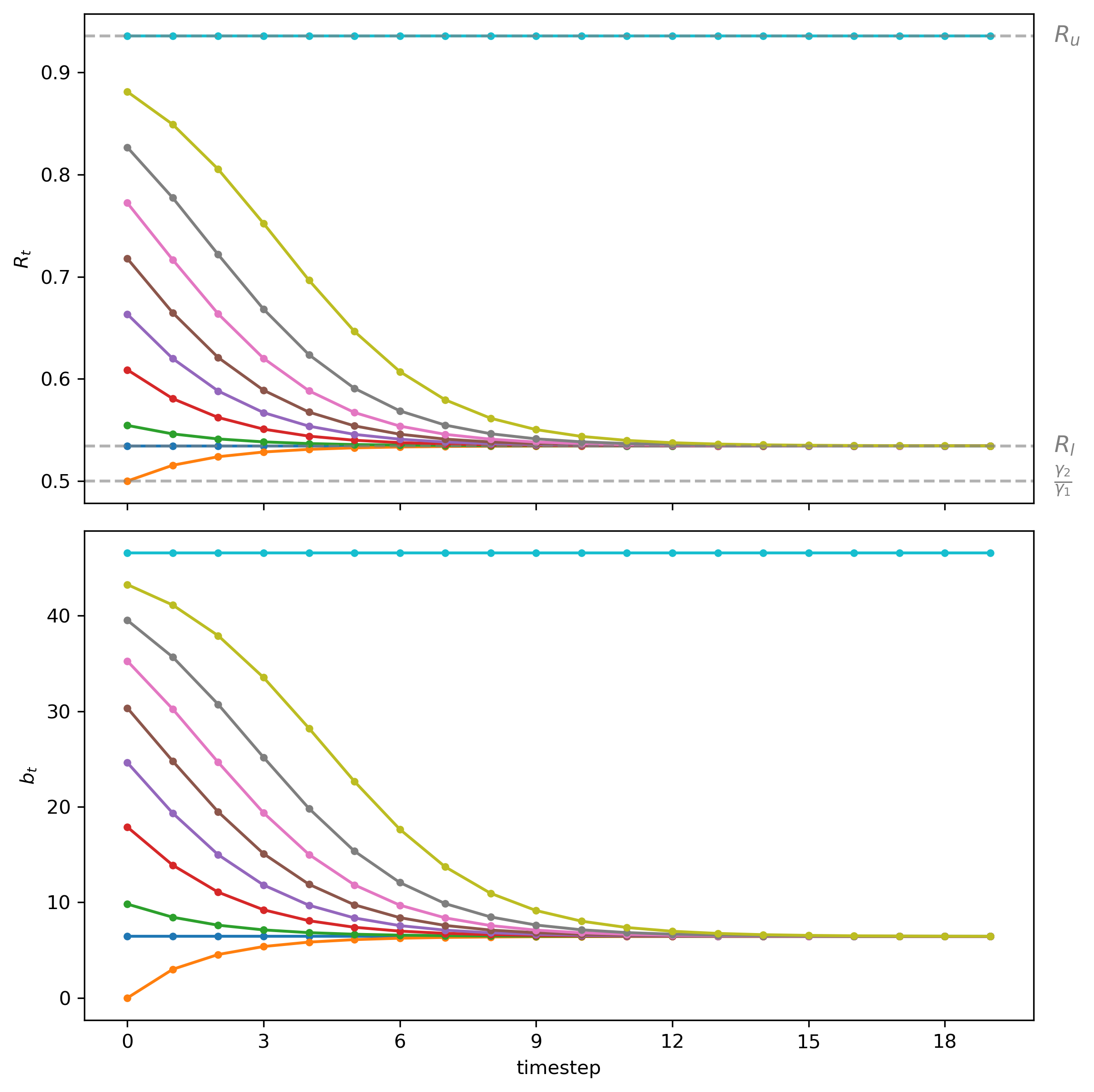
Fig. 30.2 Paths of \(R_t\) (top panel) and \(b_t\) (bottom panel) starting from different initial condition \(R_0\)#
Notice how sequences that start from \(R_0\) in the half-open interval \([R_\ell, R_u)\) converge to the steady state associated with to \( R_\ell\).
30.7. Computation method 2#
Set \(m_t = m_t^d \) for all \(t \geq -1\).
Let
Represent equilibrium conditions (30.1), (30.2), and (30.3) as
or
where
H1 = np.array([[1, msm.γ2],
               [1, 0]])
H2 = np.array([[0, msm.γ1],
               [1, msm.g]])
Define
H = np.linalg.solve(H1, H2)
print('H = \n', H)
H =
 [[ 1.    3.  ]
 [-0.02  1.94]]
and write the system (30.13) as
so that \(\{y_t\}_{t=0}\) can be computed from
where
It is natural to take \(m_0\) as an initial condition determined outside the model.
The mathematics seems to tell us that \(p_0\) must also be determined outside the model, even though it is something that we actually wanted to be determined by the model.
(As usual, we should listen when mathematics talks to us.)
For now, let’s just proceed mechanically on faith.
Compute the eigenvector decomposition
where \(\Lambda\) is a diagonal matrix of eigenvalues and the columns of \(Q\) are eigenvectors corresponding to those eigenvalues.
It turns out that
where \(R_\ell\) and \(R_u\) are the lower and higher steady-state rates of return on currency that we computed above.
Λ, Q = np.linalg.eig(H)
print('Λ = \n', Λ)
print('Q = \n', Q)
Λ =
 [1.06887658 1.87112342]
Q =
 [[-0.99973655 -0.96033288]
 [-0.02295281 -0.27885616]]
R_l = 1 / Λ[0]
R_u = 1 / Λ[1]

print(f'R_l = {R_l:.4f}')
print(f'R_u = {R_u:.4f}')
R_l = 0.9356
R_u = 0.5344
Partition \(Q\) as
Below we shall verify the following claims:
Claims: If we set
it turns out that
However, if we set
then
Let’s verify these claims step by step.
Note that
so that
def iterate_H(y_0, H, num_steps):
    Λ, Q = np.linalg.eig(H)
    Q_inv = np.linalg.inv(Q)
    y = np.stack(
        [Q @ np.diag(Λ**t) @ Q_inv @ y_0 for t in range(num_steps)], 1)

    return y
For almost all initial vectors \(y_0\), the gross rate of inflation \(\frac{p_{t+1}}{p_t}\) eventually converges to the larger eigenvalue \({R_\ell}^{-1}\).
The only way to avoid this outcome is for \(p_0\) to take the specific value described by (30.16).
To understand this situation, we use the following transformation
Dynamics of \(y^*_t\) are evidently governed by
This equation represents the dynamics of our system in a way that lets us isolate the force that causes gross inflation to converge to the inverse of the lower steady-state rate of inflation \(R_\ell\) that we discovered earlier.
Staring at equation (30.17) indicates that unless
the path of \(y^*_t\), and therefore the paths of both \(m_t\) and \(p_t\) given by \(y_t = Q y^*_t\) will eventually grow at gross rates \({R_\ell}^{-1}\) as \(t \rightarrow +\infty\).
Equation (30.18) also leads us to conclude that there is a unique setting for the initial vector \(y_0\) for which both components forever grow at the lower rate \({R_u}^{-1}\).
For this to occur, the required setting of \(y_0\) must evidently have the property that
But note that since \(y_0 = \begin{bmatrix} m_0 \cr p_0 \end{bmatrix}\) and \(m_0\) is given to us an initial condition, \(p_0\) has to do all the adjusting to satisfy this equation.
Sometimes this situation is described informally by saying that while \(m_0\) is truly a state variable, \(p_0\) is a jump variable that must adjust at \(t=0\) in order to satisfy the equation.
Thus, in a nutshell the unique value of the vector \(y_0\) for which the paths of \(y_t\) don’t eventually grow at rate \({R_\ell}^{-1}\) requires setting the second component of \(y^*_0\) equal to zero.
The component \(p_0\) of the initial vector \(y_0 = \begin{bmatrix} m_0 \cr p_0 \end{bmatrix}\) must evidently satisfy
where \(Q^{\{2\}}\) denotes the second row of \(Q^{-1}\), a restriction that is equivalent to
where \(Q^{ij}\) denotes the \((i,j)\) component of \(Q^{-1}\).
Solving this equation for \(p_0\), we find
30.7.1. More convenient formula#
We can get the equivalent but perhaps more convenient formula (30.16) for \(p_0\) that is cast in terms of components of \(Q\) instead of components of \(Q^{-1}\).
To get this formula, first note that because \((Q^{21}\ Q^{22})\) is the second row of the inverse of \(Q\) and because \(Q^{-1} Q = I\), it follows that
which implies that
Therefore,
So we can write
which is our formula (30.16).
p0_bar = (Q[1, 0]/Q[0, 0]) * msm.M0

print(f'p0_bar = {p0_bar:.4f}')
p0_bar = 2.2959
It can be verified that this formula replicates itself over time in the sense that
Now let’s visualize the dynamics of \(m_t\), \(p_t\), and \(R_t\) starting from different \(p_0\) values to verify our claims above.
We create a function draw_iterations to generate the plot
p0s = [p0_bar, 2.34, 2.5, 3, 4, 7, 30, 100_000]

draw_iterations(p0s, msm, line_params, num_steps=20)
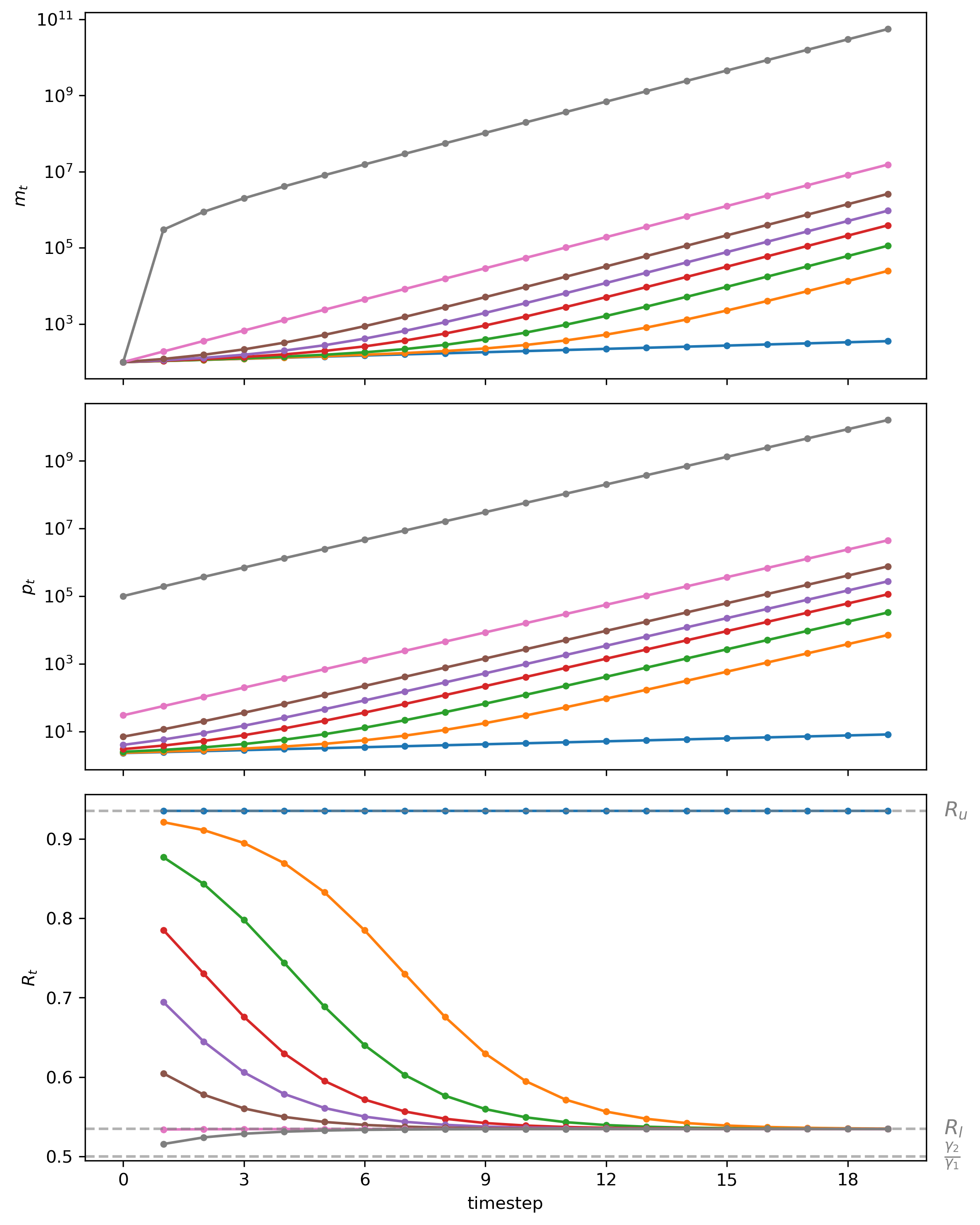
Fig. 30.3 Starting from different initial values of \(p_0\), paths of \(m_t\) (top panel, log scale for \(m\)), \(p_t\) (middle panel, log scale for \(m\)), \(R_t\) (bottom panel)#
Please notice that for \(m_t\) and \(p_t\), we have used log scales for the coordinate (i.e., vertical) axes.
Using log scales allows us to spot distinct constant limiting gross rates of growth \({R_u}^{-1}\) and \({R_\ell}^{-1}\) by eye.
30.8. Peculiar stationary outcomes#
As promised at the start of this lecture, we have encountered these concepts from macroeconomics:
an inflation tax that a government gathers by printing paper or electronic money
a dynamic Laffer curve in the inflation tax rate that has two stationary equilibria
Staring at the paths of rates of return on the price level in figure Fig. 30.2 and price levels in Fig. 30.3 show indicate that almost all paths converge to the higher inflation tax rate displayed in the stationary state Laffer curve displayed in figure Fig. 30.1.
Thus, we have indeed discovered what we earlier called “perverse” dynamics under rational expectations in which the system converges to the higher of two possible stationary inflation tax rates.
Those dynamics are “perverse” not only in the sense that they imply that the monetary and fiscal authorities that have chosen to finance government expenditures eventually impose a higher inflation tax than required to finance government expenditures, but because of the following “counterintuitive” situation that we can deduce by staring at the stationary state Laffer curve displayed in figure Fig. 30.1:
the figure indicates that inflation can be reduced by running higher government deficits, i.e., by raising more resources through printing money.
Note
The same qualitative outcomes prevail in this lecture Inflation Rate Laffer Curves that studies a nonlinear version of the model in this lecture.
30.9. Equilibrium selection#
We have discovered that as a model of price level paths or model is incomplete because there is a continuum of “equilibrium” paths for \(\{m_{t+1}, p_t\}_{t=0}^\infty\) that are consistent with the demand for real balances always equaling the supply.
Through application of our computational methods 1 and 2, we have learned that this continuum can be indexed by choice of one of two scalars:
for computational method 1, \(R_0\)
for computational method 2, \(p_0\)
To apply our model, we have somehow to complete it by selecting an equilibrium path from among the continuum of possible paths.
We discovered that
all but one of the equilibrium paths converge to limits in which the higher of two possible stationary inflation tax prevails
there is a unique equilibrium path associated with “plausible” statements about how reductions in government deficits affect a stationary inflation rate
On grounds of plausibility, we recommend following many macroeconomists in selecting the unique equilibrium that converges to the lower stationary inflation tax rate.
As we shall see, we shall accept this recommendation in lecture Some Unpleasant Monetarist Arithmetic.
In lecture, Laffer Curves with Adaptive Expectations, we shall explore how [Bruno and Fischer, 1990] and others justified this in other ways.
30.10. Exercises#
Exercise 30.1
The seigniorage Laffer curve: peak revenue and fiscal limits.
The lecture states that steady-state seigniorage
is maximized at \(\bar R_{\rm max} = \sqrt{\gamma_2/\gamma_1}\).
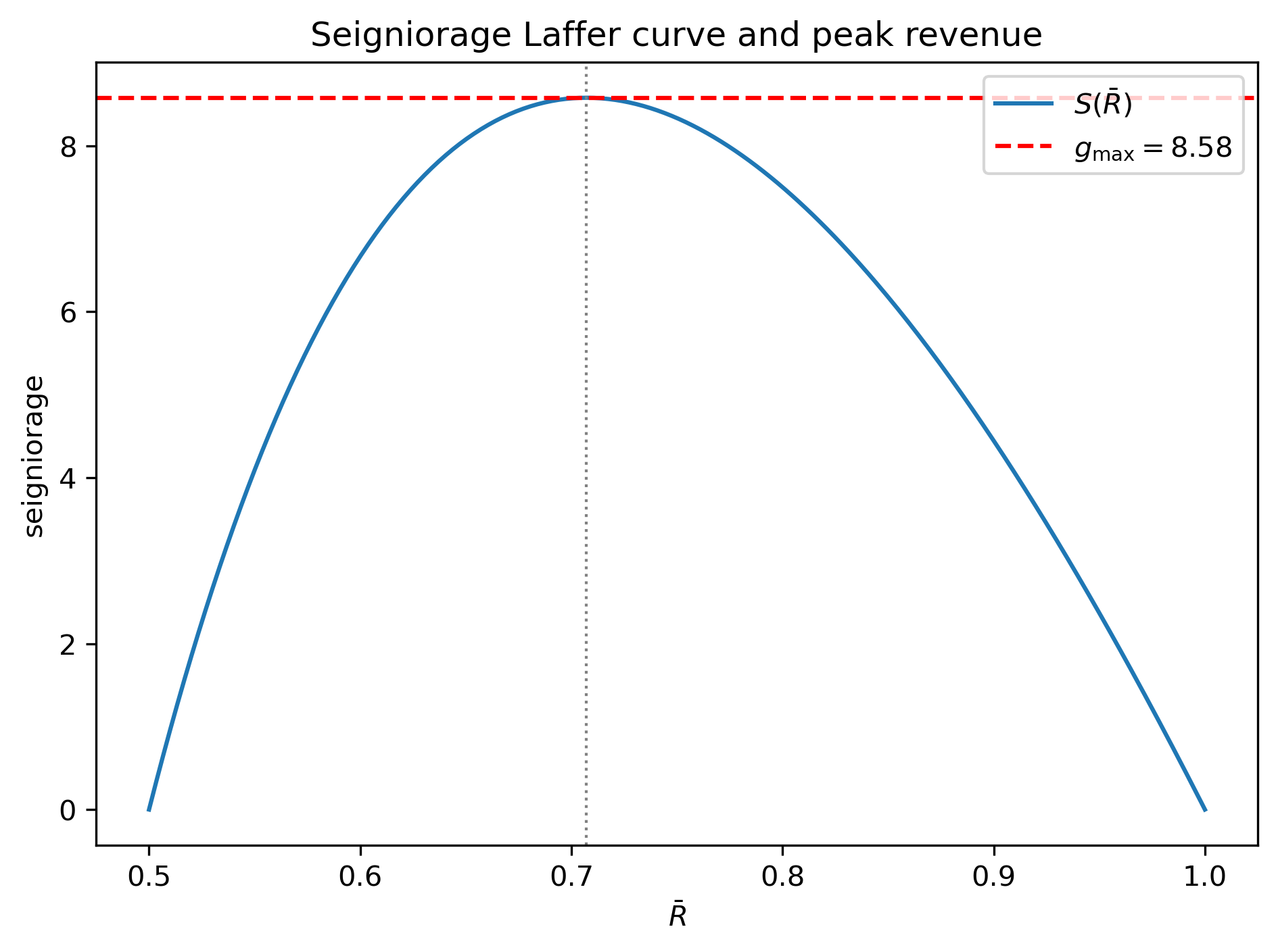
a. Verify this analytically by differentiating \(S(\bar R)\) with respect to \(\bar R\), setting the derivative to zero, and solving for \(\bar R\).
b. Using the default model msm, compute \(\bar R_{\rm max}\) and the
corresponding maximum revenue \(g_{\rm max} = S(\bar R_{\rm max})\), then
plot the seigniorage curve together with a horizontal line at \(g_{\rm max}\).
c. Evaluate the discriminant of the steady-state quadratic (30.9) for \(g = g_{\rm max} + 1\) and explain what happens if the government tries to finance a deficit \(g > g_{\rm max}\).
Solution to Exercise 30.1
Part a. Differentiating with respect to \(\bar R\):
Since \(S''(\bar R) = -2\gamma_2/\bar R^3 < 0\), this is indeed a maximum.
γ1, γ2 = msm.γ1, msm.γ2

R_max = np.sqrt(γ2 / γ1)
g_max = seign(R_max, msm)
print(f"R_max = sqrt(γ2/γ1) = sqrt({γ2}/{γ1}) = {R_max:.4f}")
print(f"g_max = S(R_max)     = {g_max:.4f}")

R_plot = np.linspace(γ2/γ1, 1, 300)
fig, ax = plt.subplots()
ax.plot(R_plot, seign(R_plot, msm), label='$S(\\bar R)$')
ax.axhline(g_max, color='red', linestyle='--', label=f'$g_{{\\rm max}}={g_max:.2f}$')
ax.axvline(R_max, color='grey', linestyle=':', lw=1)
ax.set_xlabel('$\\bar R$')
ax.set_ylabel('seigniorage')
ax.set_title('Seigniorage Laffer curve and peak revenue')
ax.legend()
plt.tight_layout()
plt.show()
R_max = sqrt(γ2/γ1) = sqrt(50/100) = 0.7071
g_max = S(R_max)     = 8.5786
Part c. The steady-state quadratic is \(-\gamma_1 \bar R^2 + (\gamma_1+\gamma_2-g)\bar R - \gamma_2 = 0\).
Its discriminant is \((\gamma_1+\gamma_2-g)^2 - 4\gamma_1\gamma_2\).
g_too_high = g_max + 1
discriminant = (γ1 + γ2 - g_too_high)**2 - 4 * γ1 * γ2
roots = np.roots((-γ1, γ1 + γ2 - g_too_high, -γ2))
print(f"g = g_max + 1 = {g_too_high:.4f}")
print(f"Discriminant  = {discriminant:.4f}  ({'negative' if discriminant < 0 else 'positive'})")
print(f"np.roots      = {roots}")
print(f"Roots are real: {np.all(np.isreal(roots))}")
g = g_max + 1 = 9.5786
Discriminant  = -281.8427  (negative)
np.roots      = [0.70210678+0.08394086j 0.70210678-0.08394086j]
Roots are real: False
When \(g > g_{\rm max}\) the discriminant is negative and there are no real steady-state rates of return on currency.
Economically, the government is trying to finance a deficit that exceeds the maximum amount of seigniorage the inflation tax can ever raise, regardless of the inflation rate chosen.
No stationary equilibrium exists.
Exercise 30.2
How steady-state rates of return vary with the government deficit.
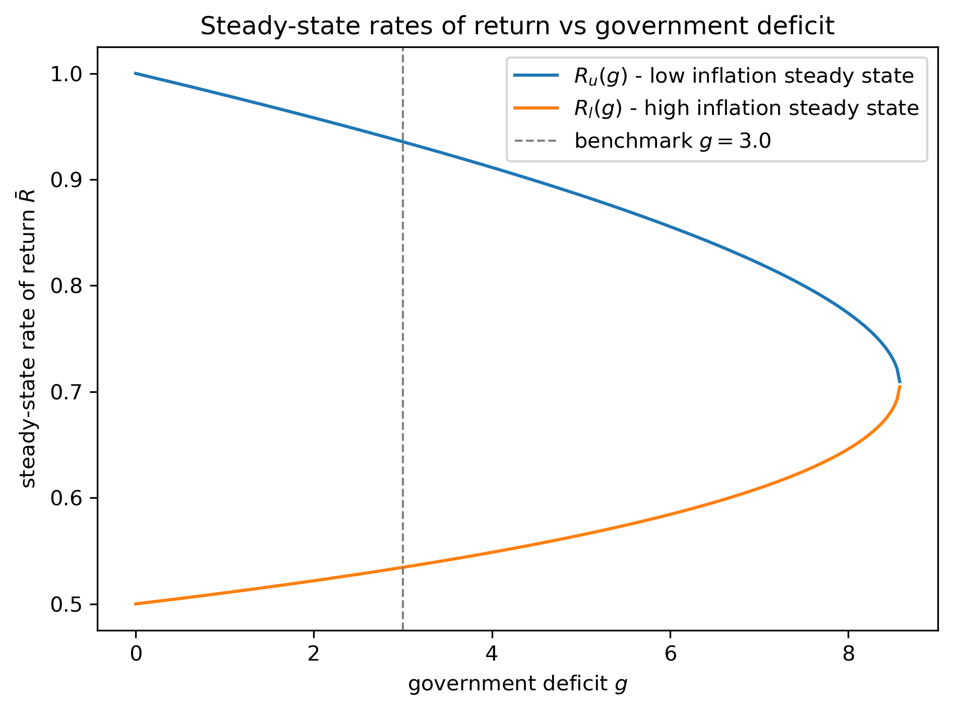
The two steady-state roots \(R_l < R_u\) of the quadratic (30.9) depend on the government deficit \(g\).
a. For \(g\) ranging from a value near \(0\) to just below \(g_{\rm max}\), compute both roots \(R_l(g)\) and \(R_u(g)\) and plot them against \(g\) on the same graph.
b. Verify the following boundary conditions analytically and numerically:
* At $g = 0$: the two roots should be $R = 1$ and $R = \gamma_2/\gamma_1$.
* As $g \to g_{\rm max}$: the two roots should merge at $\bar R_{\rm max} = \sqrt{\gamma_2/\gamma_1}$.
c. Mark the benchmark deficit \(g = 3\) on your graph, read off \(R_u\) and \(R_l\),
and check whether your graph values agree with msm.R_u and msm.R_l.
Solution to Exercise 30.2
R_max = np.sqrt(msm.γ2 / msm.γ1)
g_max = seign(R_max, msm)

g_grid = np.linspace(1e-6, g_max * (1 - 1e-4), 300)
R_u_curve, R_l_curve = [], []

for g in g_grid:
    roots = np.sort(np.roots((-msm.γ1, msm.γ1 + msm.γ2 - g, -msm.γ2)).real)
    R_l_curve.append(roots[0])
    R_u_curve.append(roots[1])

fig, ax = plt.subplots()
ax.plot(g_grid, R_u_curve, label='$R_u(g)$ - low inflation steady state')
ax.plot(g_grid, R_l_curve, label='$R_l(g)$ - high inflation steady state')
ax.axvline(msm.g, color='grey', linestyle='--', lw=1,
           label=f'benchmark $g = {msm.g}$')
ax.set_xlabel('government deficit $g$')
ax.set_ylabel('steady-state rate of return $\\bar R$')
ax.set_title('Steady-state rates of return vs government deficit')
ax.legend()
plt.tight_layout()
plt.show()

# Boundary conditions
print("Boundary checks:")
print(f"  g -> 0:     R_u -> {R_u_curve[0]:.4f}  (expected 1.0)")
print(f"              R_l -> {R_l_curve[0]:.4f}  (expected γ2/γ1 = {msm.γ2/msm.γ1:.4f})")
print(f"  g -> g_max: R_u -> {R_u_curve[-1]:.4f}")
print(f"              R_l -> {R_l_curve[-1]:.4f}")
print(f"             R_max = {R_max:.4f}  (roots should merge here)")
print(f"\nAt benchmark g = {msm.g}:")
print(f"  R_u from curve = {R_u_curve[np.argmin(np.abs(g_grid - msm.g))]:.4f},  "
      f"msm.R_u = {msm.R_u:.4f}")
print(f"  R_l from curve = {R_l_curve[np.argmin(np.abs(g_grid - msm.g))]:.4f},  "
      f"msm.R_l = {msm.R_l:.4f}")
Boundary checks:
  g -> 0:     R_u -> 1.0000  (expected 1.0)
              R_l -> 0.5000  (expected γ2/γ1 = 0.5000)
  g -> g_max: R_u -> 0.7096
              R_l -> 0.7046
             R_max = 0.7071  (roots should merge here)

At benchmark g = 3.0:
  R_u from curve = 0.9353,  msm.R_u = 0.9356
  R_l from curve = 0.5346,  msm.R_l = 0.5344
The two branches of the Laffer curve start apart at \(g=0\) and merge at \(g = g_{\rm max}\).
For \(g > g_{\rm max}\) no real steady state exists.
The upper branch \(R_u(g)\) falls and the lower branch \(R_l(g)\) rises as \(g\) increases, reflecting the increasing inflation tax needed to finance a larger deficit.
Exercise 30.3
Quantity theory of money via the eigendecomposition.
Method 2 identifies a unique “magic” initial price level
(where \(Q_{ij}\) denotes the \((i,j)\) element of the eigenvector matrix \(Q\)) that places the economy on the low-inflation equilibrium path.
a. Using iterate_H, simulate the path of \(y_t = (m_t, p_t)\) starting from
\(y_0 = (m_0,\, \bar p_0)\), compute \(R_t = p_t/p_{t+1}\) for \(t = 0, \ldots, 10\),
and verify that it equals msm.R_u at every step.
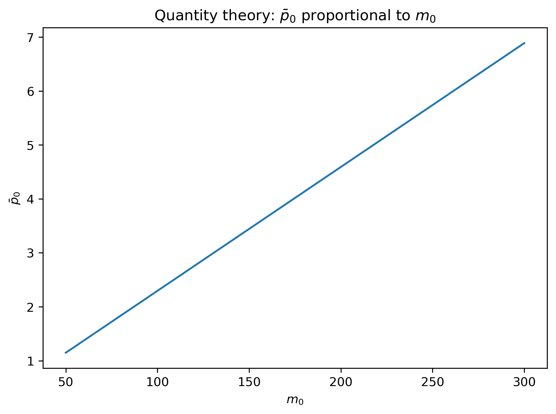
b. Use the formula \(\bar p_0 = (Q_{21}/Q_{11})\, m_0\) to interpret the initial price level as proportional to the money supply, compute \(\bar p_0\) for \(m_0 \in [50, 300]\), plot \(\bar p_0\) against \(m_0\), and report the slope.
c. Set \(R_0 = R_u\) in the Method 1 formula for \(p_0\) from equation (30.11) and confirm that you recover \(\bar p_0\).
Solution to Exercise 30.3
# Part a: verify R_t = R_u along the magic-p0 path
p0_bar = (Q[1, 0] / Q[0, 0]) * msm.M0
y0 = np.array([msm.M0, p0_bar])
num_steps = 12

y_series = iterate_H(y0, H, num_steps)
P = y_series[1, :]
R_path = P[:-1] / P[1:]      # R_t = p_t / p_{t+1}

print(f"R_t along the magic-p0 path (first {num_steps-1} periods):")
print(np.round(R_path, 6))
print(f"msm.R_u = {msm.R_u:.6f}")
R_t along the magic-p0 path (first 11 periods):
[0.935562 0.935562 0.935562 0.935562 0.935562 0.935562 0.935562 0.935562
 0.935562 0.935562 0.935562]
msm.R_u = 0.935562
# Part b: plot p0_bar vs m0
m0_values = np.linspace(50, 300, 80)
p0_bar_values = (Q[1, 0] / Q[0, 0]) * m0_values

fig, ax = plt.subplots()
ax.plot(m0_values, p0_bar_values)
ax.set_xlabel('$m_0$')
ax.set_ylabel('$\\bar p_0$')
ax.set_title('Quantity theory: $\\bar p_0$ proportional to $m_0$')
plt.tight_layout()
plt.show()

slope = Q[1, 0] / Q[0, 0]
print(f"Slope = Q_21 / Q_11 = {slope:.6f}")

# Part c: compare with Method 1 formula eq:p0fromR0
p0_method1 = msm.M0 / (msm.γ1 - msm.g - msm.γ2 / msm.R_u)
print(f"\nMethod 1 formula (R_0 = R_u):  p0 = {p0_method1:.6f}")
print(f"Eigendecomposition formula:    p0 = {p0_bar:.6f}")
Slope = Q_21 / Q_11 = 0.022959

Method 1 formula (R_0 = R_u):  p0 = 2.295886
Eigendecomposition formula:    p0 = 2.295886
Parts a and c confirm that both methods select exactly the same unique initial price level.
Part b shows the quantity-theory proportionality that doubling \(m_0\) exactly doubles \(\bar p_0\), with constant slope \(Q_{21}/Q_{11}\).
This linearity is a direct consequence of the linearity of the model.