19. Probability Distributions#
19.1. Outline#
In data science applications, we are often interested in data on a specific variable.
In this lecture we give a quick introduction to data and probability distributions using Python.
!pip install --upgrade yfinance
import matplotlib.pyplot as plt
import pandas as pd
import numpy as np
import yfinance as yf
import scipy.stats
import seaborn as sns
To motivate what follows, let’s start with a real example: the heights of adult men and women in the United States.
The data come from the US National Health and Nutrition Examination Survey (NHANES).
The next figure shows histograms of the two datasets, with heights measured in centimeters.
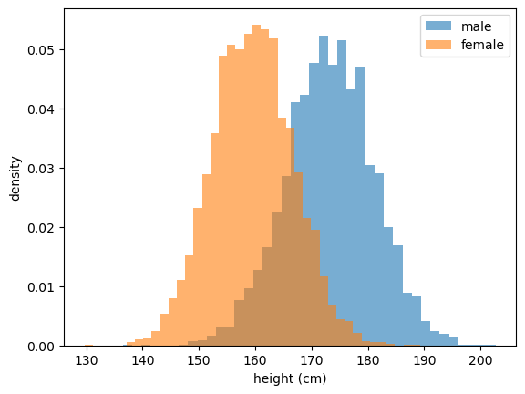
Fig. 19.1 Heights of US adults (NHANES)#
Each histogram has the familiar “bell” shape.
This suggests that we can approximate the data using a normal distribution — a continuous distribution with a bell-shaped density that we study in detail below.
To do so, we fit a normal distribution to each dataset, choosing its mean and standard deviation to match the sample mean and standard deviation of the heights.
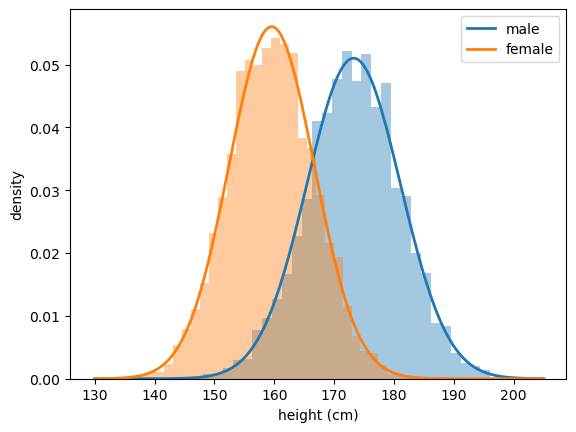
Fig. 19.2 Normal fit to US adult heights#
The fit is remarkably good.
Notice what this achieves: each dataset of around 5,000 individual measurements is now summarized by a smooth density with just two parameters — the mean \(\mu\), which sets the center, and the standard deviation \(\sigma\), which sets the spread.
Such compact summaries are extremely useful.
They are one reason we study common distributions: named families of distributions, each governed by a small number of parameters, that have proven useful for describing data.
We turn to these now.
19.2. Common distributions#
In this section we recall the definitions of some well-known distributions and explore how to manipulate them with SciPy.
19.2.1. Discrete distributions#
Let’s start with discrete distributions.
A discrete distribution is defined by a set of numbers \(S = \{x_1, \ldots, x_n\}\) and a probability mass function (PMF) on \(S\), which is a function \(p\) from \(S\) to \([0,1]\) with the property
For example, the next figure shows the fraction of people at each age in Japan in 2024 (Japanese nationals), from 0 to 100 and over.
The data come from the Statistics Bureau of Japan.
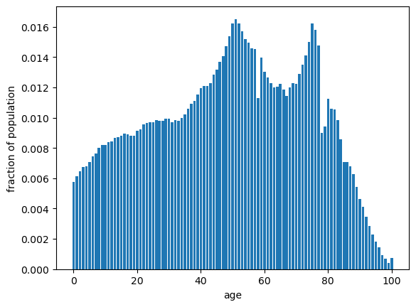
Fig. 19.3 Population share by age, Japan 2024#
Here each \(x_i\) is an age and \(p(x_i)\) is the fraction of the population at that age, and the fractions sum to one.
We say that a random variable \(X\) has distribution \(p\) if \(X\) takes value \(x_i\) with probability \(p(x_i)\).
That is,
The mean or expected value of a random variable \(X\) with distribution \(p\) is
Expectation is also called the first moment of the distribution.
We also refer to this number as the mean of the distribution (represented by) \(p\).
The variance of \(X\) is defined as
Variance is also called the second central moment of the distribution.
The cumulative distribution function (CDF) of \(X\) is defined by
Here \(\mathbb 1\{ \textrm{statement} \} = 1\) if “statement” is true and zero otherwise.
Hence the second term takes all \(x_i \leq x\) and sums their probabilities.
19.2.1.1. Uniform distribution#
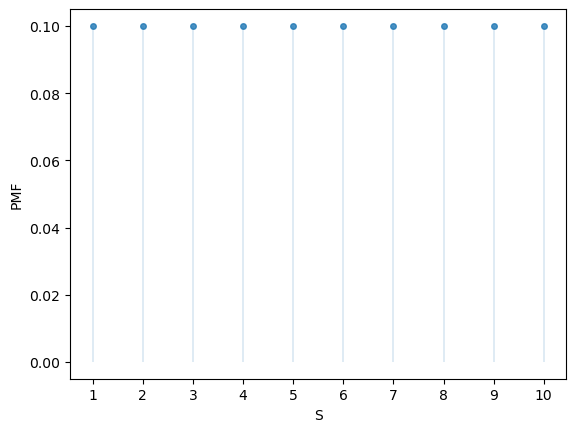
One simple example is the uniform distribution, where \(p(x_i) = 1/n\) for all \(i\).
We can import the uniform distribution on \(S = \{1, \ldots, n\}\) from SciPy like so:
n = 10
u = scipy.stats.randint(1, n+1)
Here’s the mean and variance:
u.mean(), u.var()
(np.float64(5.5), np.float64(8.25))
The formula for the mean is \((n+1)/2\), and the formula for the variance is \((n^2 - 1)/12\).
Now let’s evaluate the PMF:
u.pmf(1)
np.float64(0.1)
u.pmf(2)
np.float64(0.1)
Here’s a plot of the probability mass function:
fig, ax = plt.subplots()
S = np.arange(1, n+1)
ax.plot(S, u.pmf(S), linestyle='', marker='o', alpha=0.8, ms=4)
ax.vlines(S, 0, u.pmf(S), lw=0.2)
ax.set_xticks(S)
ax.set_xlabel('S')
ax.set_ylabel('PMF')
plt.show()
Here’s a plot of the CDF:
fig, ax = plt.subplots()
S = np.arange(1, n+1)
ax.step(S, u.cdf(S))
ax.vlines(S, 0, u.cdf(S), lw=0.2)
ax.set_xticks(S)
ax.set_xlabel('S')
ax.set_ylabel('CDF')
plt.show()
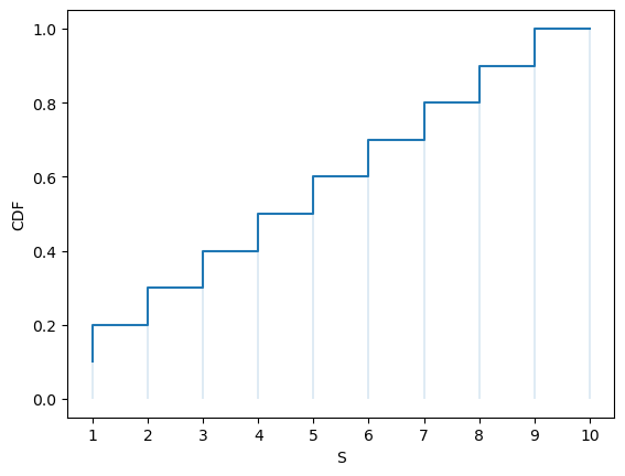
The CDF jumps up by \(p(x_i)\) at \(x_i\).
Exercise 19.1
Calculate the mean and variance for this parameterization (i.e., \(n=10\)) directly from the PMF, using the expressions given above.
Check that your answers agree with u.mean() and u.var().
19.2.1.2. Bernoulli distribution#
Another useful distribution is the Bernoulli distribution on \(S = \{0,1\}\), which has PMF:
Here \(\theta \in [0,1]\) is a parameter.
We can think of this distribution as modeling probabilities for a random trial with success probability \(\theta\).
\(p(1) = \theta\) means that the trial succeeds (takes value 1) with probability \(\theta\)
\(p(0) = 1 - \theta\) means that the trial fails (takes value 0) with probability \(1-\theta\)
The formula for the mean is \(\theta\), and the formula for the variance is \(\theta(1-\theta)\).
We can import the Bernoulli distribution on \(S = \{0,1\}\) from SciPy like so:
θ = 0.4
u = scipy.stats.bernoulli(θ)
Here’s the mean and variance at \(\theta=0.4\)
u.mean(), u.var()
(np.float64(0.4), np.float64(0.24))
We can evaluate the PMF as follows
u.pmf(0), u.pmf(1)
(np.float64(0.6), np.float64(0.4))
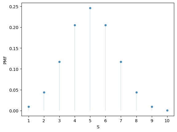
19.2.1.3. Binomial distribution#
Another useful (and more interesting) distribution is the binomial distribution on \(S=\{0, \ldots, n\}\), which has PMF:
Again, \(\theta \in [0,1]\) is a parameter.
The interpretation of \(p(i)\) is: the probability of \(i\) successes in \(n\) independent trials with success probability \(\theta\).
For example, if \(\theta=0.5\), then \(p(i)\) is the probability of \(i\) heads in \(n\) flips of a fair coin.
The formula for the mean is \(n \theta\) and the formula for the variance is \(n \theta (1-\theta)\).
Let’s investigate an example
n = 10
θ = 0.5
u = scipy.stats.binom(n, θ)
According to our formulas, the mean and variance are
n * θ, n * θ * (1 - θ)
(5.0, 2.5)
Let’s see if SciPy gives us the same results:
u.mean(), u.var()
(np.float64(5.0), np.float64(2.5))
Here’s the PMF:
u.pmf(1)
np.float64(0.009765625000000002)
fig, ax = plt.subplots()
S = np.arange(1, n+1)
ax.plot(S, u.pmf(S), linestyle='', marker='o', alpha=0.8, ms=4)
ax.vlines(S, 0, u.pmf(S), lw=0.2)
ax.set_xticks(S)
ax.set_xlabel('S')
ax.set_ylabel('PMF')
plt.show()
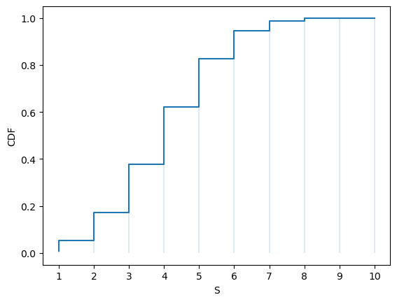
Here’s the CDF:
fig, ax = plt.subplots()
S = np.arange(1, n+1)
ax.step(S, u.cdf(S))
ax.vlines(S, 0, u.cdf(S), lw=0.2)
ax.set_xticks(S)
ax.set_xlabel('S')
ax.set_ylabel('CDF')
plt.show()

Exercise 19.2
Using u.pmf, check that our definition of the CDF given above calculates the same function as u.cdf.
Solution
Here is one solution:
fig, ax = plt.subplots()
S = np.arange(1, n+1)
u_sum = np.cumsum(u.pmf(S))
ax.step(S, u_sum)
ax.vlines(S, 0, u_sum, lw=0.2)
ax.set_xticks(S)
ax.set_xlabel('S')
ax.set_ylabel('CDF')
plt.show()
We can see that the output graph is the same as the one above.
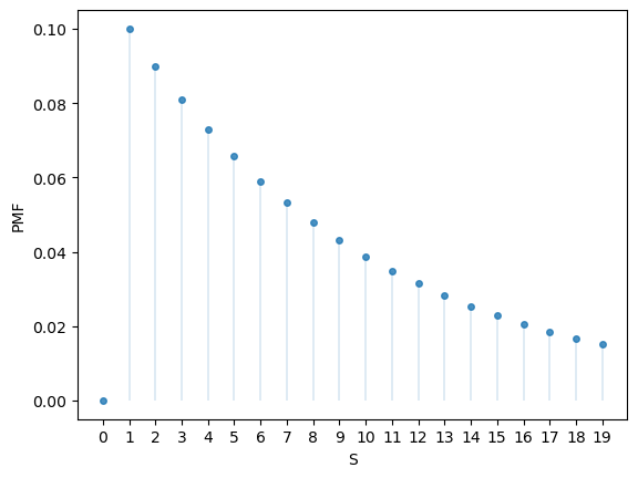
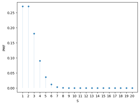
19.2.1.4. Geometric distribution#
The geometric distribution has infinite support \(S = \{0, 1, 2, \ldots\}\) and its PMF is given by
where \(\theta \in [0,1]\) is a parameter
(A discrete distribution has infinite support if the set of points to which it assigns positive probability is infinite.)
To understand the distribution, think of repeated independent random trials, each with success probability \(\theta\).
The interpretation of \(p(i)\) is: the probability there are \(i\) failures before the first success occurs.
It can be shown that the mean of the distribution is \(1/\theta\) and the variance is \((1-\theta)/\theta\).
Here’s an example.
θ = 0.1
u = scipy.stats.geom(θ)
u.mean(), u.var()
(np.float64(10.0), np.float64(90.0))
Here’s part of the PMF:
fig, ax = plt.subplots()
n = 20
S = np.arange(n)
ax.plot(S, u.pmf(S), linestyle='', marker='o', alpha=0.8, ms=4)
ax.vlines(S, 0, u.pmf(S), lw=0.2)
ax.set_xticks(S)
ax.set_xlabel('S')
ax.set_ylabel('PMF')
plt.show()
19.2.1.5. Poisson distribution#
The Poisson distribution on \(S = \{0, 1, \ldots\}\) with parameter \(\lambda > 0\) has PMF
The interpretation of \(p(i)\) is: the probability of \(i\) events in a fixed time interval, where the events occur independently at a constant rate \(\lambda\).
It can be shown that the mean is \(\lambda\) and the variance is also \(\lambda\).
Here’s an example.
λ = 2
u = scipy.stats.poisson(λ)
u.mean(), u.var()
(np.float64(2.0), np.float64(2.0))
Here’s the PMF:
u.pmf(1)
np.float64(0.2706705664732254)
fig, ax = plt.subplots()
S = np.arange(1, n+1)
ax.plot(S, u.pmf(S), linestyle='', marker='o', alpha=0.8, ms=4)
ax.vlines(S, 0, u.pmf(S), lw=0.2)
ax.set_xticks(S)
ax.set_xlabel('S')
ax.set_ylabel('PMF')
plt.show()
19.2.2. Continuous distributions#
A continuous distribution is represented by a probability density function, which is a function \(p\) over \(\mathbb R\) (the set of all real numbers) such that \(p(x) \geq 0\) for all \(x\) and
We say that random variable \(X\) has distribution \(p\) if
for all \(a \leq b\).
The definition of the mean and variance of a random variable \(X\) with distribution \(p\) are the same as the discrete case, after replacing the sum with an integral.
For example, the mean of \(X\) is
The cumulative distribution function (CDF) of \(X\) is defined by
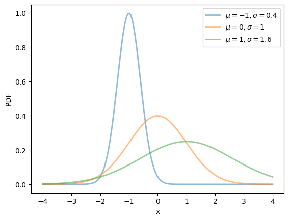
19.2.2.1. Normal distribution#
Perhaps the most famous distribution is the normal distribution, which has density
This distribution has two parameters, \(\mu \in \mathbb R\) and \(\sigma \in (0, \infty)\).
Using calculus, it can be shown that, for this distribution, the mean is \(\mu\) and the variance is \(\sigma^2\).
We can obtain the moments, PDF and CDF of the normal density via SciPy as follows:
μ, σ = 0.0, 1.0
u = scipy.stats.norm(μ, σ)
u.mean(), u.var()
(np.float64(0.0), np.float64(1.0))
Here’s a plot of the density — the famous “bell-shaped curve”:
μ_vals = [-1, 0, 1]
σ_vals = [0.4, 1, 1.6]
fig, ax = plt.subplots()
x_grid = np.linspace(-4, 4, 200)

for μ, σ in zip(μ_vals, σ_vals):
    u = scipy.stats.norm(μ, σ)
    ax.plot(x_grid, u.pdf(x_grid),
    alpha=0.5, lw=2,
    label=rf'$\mu={μ}, \sigma={σ}$')
ax.set_xlabel('x')
ax.set_ylabel('PDF')
plt.legend()
plt.show()
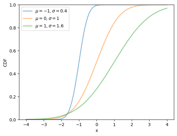
Here’s a plot of the CDF:
fig, ax = plt.subplots()
for μ, σ in zip(μ_vals, σ_vals):
    u = scipy.stats.norm(μ, σ)
    ax.plot(x_grid, u.cdf(x_grid),
    alpha=0.5, lw=2,
    label=rf'$\mu={μ}, \sigma={σ}$')
    ax.set_ylim(0, 1)
ax.set_xlabel('x')
ax.set_ylabel('CDF')
plt.legend()
plt.show()
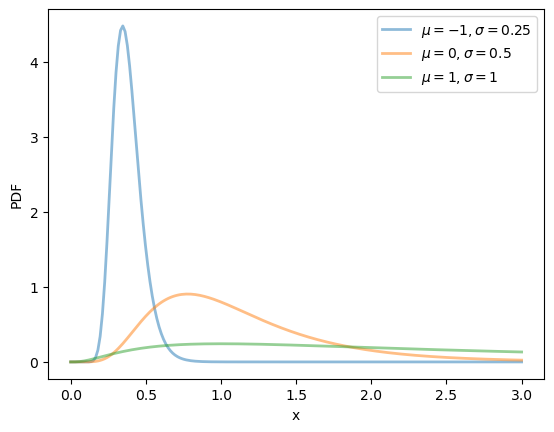
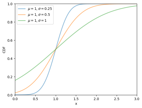
19.2.2.2. Lognormal distribution#
The lognormal distribution is a distribution on \(\left(0, \infty\right)\) with density
This distribution has two parameters, \(\mu\) and \(\sigma\).
It can be shown that, for this distribution, the mean is \(\exp\left(\mu + \sigma^2/2\right)\) and the variance is \(\left[\exp\left(\sigma^2\right) - 1\right] \exp\left(2\mu + \sigma^2\right)\).
It can be proved that
if \(X\) is lognormally distributed, then \(\log X\) is normally distributed, and
if \(X\) is normally distributed, then \(\exp X\) is lognormally distributed.
We can obtain the moments, PDF, and CDF of the lognormal density as follows:
μ, σ = 0.0, 1.0
u = scipy.stats.lognorm(s=σ, scale=np.exp(μ))
u.mean(), u.var()
(np.float64(1.6487212707001282), np.float64(4.670774270471604))
μ_vals = [-1, 0, 1]
σ_vals = [0.25, 0.5, 1]
x_grid = np.linspace(0, 3, 200)

fig, ax = plt.subplots()
for μ, σ in zip(μ_vals, σ_vals):
    u = scipy.stats.lognorm(σ, scale=np.exp(μ))
    ax.plot(x_grid, u.pdf(x_grid),
    alpha=0.5, lw=2,
    label=fr'$\mu={μ}, \sigma={σ}$')
ax.set_xlabel('x')
ax.set_ylabel('PDF')
plt.legend()
plt.show()
fig, ax = plt.subplots()
μ = 1
for σ in σ_vals:
    u = scipy.stats.norm(μ, σ)
    ax.plot(x_grid, u.cdf(x_grid),
    alpha=0.5, lw=2,
    label=rf'$\mu={μ}, \sigma={σ}$')
    ax.set_ylim(0, 1)
    ax.set_xlim(0, 3)
ax.set_xlabel('x')
ax.set_ylabel('CDF')
plt.legend()
plt.show()
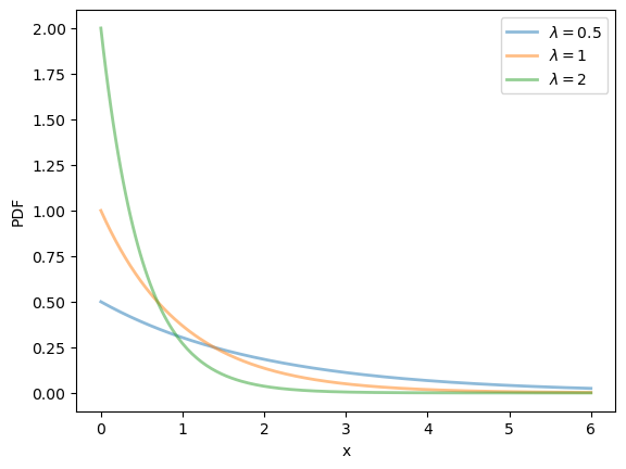
19.2.2.3. Exponential distribution#
The exponential distribution is a distribution supported on \(\left(0, \infty\right)\) with density
This distribution has one parameter \(\lambda\).
The exponential distribution can be thought of as the continuous analog of the geometric distribution.
It can be shown that, for this distribution, the mean is \(1/\lambda\) and the variance is \(1/\lambda^2\).
We can obtain the moments, PDF, and CDF of the exponential density as follows:
λ = 1.0
u = scipy.stats.expon(scale=1/λ)
u.mean(), u.var()
(np.float64(1.0), np.float64(1.0))
fig, ax = plt.subplots()
λ_vals = [0.5, 1, 2]
x_grid = np.linspace(0, 6, 200)

for λ in λ_vals:
    u = scipy.stats.expon(scale=1/λ)
    ax.plot(x_grid, u.pdf(x_grid),
    alpha=0.5, lw=2,
    label=rf'$\lambda={λ}$')
ax.set_xlabel('x')
ax.set_ylabel('PDF')
plt.legend()
plt.show()
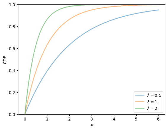
fig, ax = plt.subplots()
for λ in λ_vals:
    u = scipy.stats.expon(scale=1/λ)
    ax.plot(x_grid, u.cdf(x_grid),
    alpha=0.5, lw=2,
    label=rf'$\lambda={λ}$')
    ax.set_ylim(0, 1)
ax.set_xlabel('x')
ax.set_ylabel('CDF')
plt.legend()
plt.show()
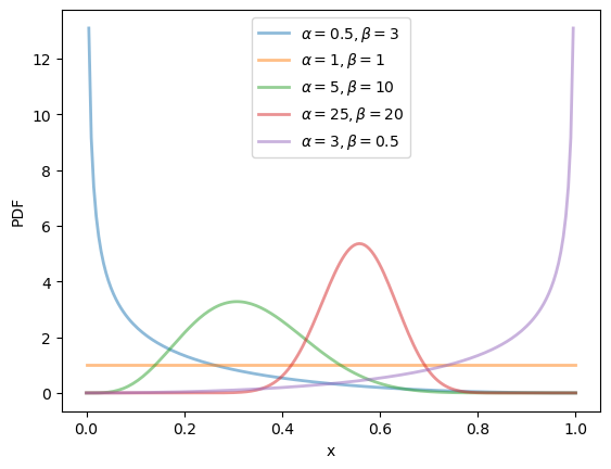
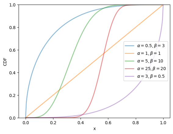
19.2.2.4. Beta distribution#
The beta distribution is a distribution on \((0, 1)\) with density
where \(\Gamma\) is the gamma function.
(The role of the gamma function is just to normalize the density, so that it integrates to one.)
This distribution has two parameters, \(\alpha > 0\) and \(\beta > 0\).
It can be shown that, for this distribution, the mean is \(\alpha / (\alpha + \beta)\) and the variance is \(\alpha \beta / (\alpha + \beta)^2 (\alpha + \beta + 1)\).
We can obtain the moments, PDF, and CDF of the Beta density as follows:
α, β = 3.0, 1.0
u = scipy.stats.beta(α, β)
u.mean(), u.var()
(np.float64(0.75), np.float64(0.0375))
α_vals = [0.5, 1, 5, 25, 3]
β_vals = [3, 1, 10, 20, 0.5]
x_grid = np.linspace(0, 1, 200)

fig, ax = plt.subplots()
for α, β in zip(α_vals, β_vals):
    u = scipy.stats.beta(α, β)
    ax.plot(x_grid, u.pdf(x_grid),
    alpha=0.5, lw=2,
    label=rf'$\alpha={α}, \beta={β}$')
ax.set_xlabel('x')
ax.set_ylabel('PDF')
plt.legend()
plt.show()
fig, ax = plt.subplots()
for α, β in zip(α_vals, β_vals):
    u = scipy.stats.beta(α, β)
    ax.plot(x_grid, u.cdf(x_grid),
    alpha=0.5, lw=2,
    label=rf'$\alpha={α}, \beta={β}$')
    ax.set_ylim(0, 1)
ax.set_xlabel('x')
ax.set_ylabel('CDF')
plt.legend()
plt.show()
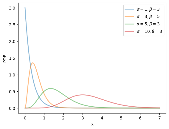
19.2.2.5. Gamma distribution#
The gamma distribution is a distribution on \(\left(0, \infty\right)\) with density
This distribution has two parameters, \(\alpha > 0\) and \(\beta > 0\).
It can be shown that, for this distribution, the mean is \(\alpha / \beta\) and the variance is \(\alpha / \beta^2\).
One interpretation is that if \(X\) is gamma distributed and \(\alpha\) is an integer, then \(X\) is the sum of \(\alpha\) independent exponentially distributed random variables with mean \(1/\beta\).
We can obtain the moments, PDF, and CDF of the Gamma density as follows:
α, β = 3.0, 2.0
u = scipy.stats.gamma(α, scale=1/β)
u.mean(), u.var()
(np.float64(1.5), np.float64(0.75))
α_vals = [1, 3, 5, 10]
β_vals = [3, 5, 3, 3]
x_grid = np.linspace(0, 7, 200)

fig, ax = plt.subplots()
for α, β in zip(α_vals, β_vals):
    u = scipy.stats.gamma(α, scale=1/β)
    ax.plot(x_grid, u.pdf(x_grid),
    alpha=0.5, lw=2,
    label=rf'$\alpha={α}, \beta={β}$')
ax.set_xlabel('x')
ax.set_ylabel('PDF')
plt.legend()
plt.show()
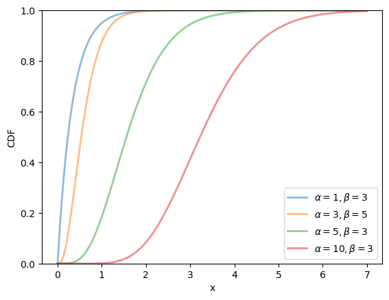
fig, ax = plt.subplots()
for α, β in zip(α_vals, β_vals):
    u = scipy.stats.gamma(α, scale=1/β)
    ax.plot(x_grid, u.cdf(x_grid),
    alpha=0.5, lw=2,
    label=rf'$\alpha={α}, \beta={β}$')
    ax.set_ylim(0, 1)
ax.set_xlabel('x')
ax.set_ylabel('CDF')
plt.legend()
plt.show()
19.3. Observed distributions#
Sometimes we refer to observed data or measurements as “distributions”.
For example, let’s say we observe the income of 10 people over a year:
data = [['Hiroshi', 1200],
        ['Ako', 1210],
        ['Emi', 1400],
        ['Daiki', 990],
        ['Chiyo', 1530],
        ['Taka', 1210],
        ['Katsuhiko', 1240],
        ['Daisuke', 1124],
        ['Yoshi', 1330],
        ['Rie', 1340]]

df = pd.DataFrame(data, columns=['name', 'income'])
df
| name | income | |
|---|---|---|
| 0 | Hiroshi | 1200 |
| 1 | Ako | 1210 |
| 2 | Emi | 1400 |
| 3 | Daiki | 990 |
| 4 | Chiyo | 1530 |
| 5 | Taka | 1210 |
| 6 | Katsuhiko | 1240 |
| 7 | Daisuke | 1124 |
| 8 | Yoshi | 1330 |
| 9 | Rie | 1340 |
In this situation, we might refer to the set of their incomes as the “income distribution.”
The terminology is confusing because this set is not a probability distribution — it’s just a collection of numbers.
However, as we will see, there are connections between observed distributions (i.e., sets of numbers like the income distribution above) and probability distributions.
Below we explore some observed distributions.
19.3.1. Summary statistics#
Suppose we have an observed distribution with values \(\{x_1, \ldots, x_n\}\)
The sample mean of this distribution is defined as
The sample variance is defined as
For the income distribution given above, we can calculate these numbers via
x = df['income']
x.mean(), x.var()
(np.float64(1257.4), np.float64(22680.93333333333))
Exercise 19.3
If you try to check that the formulas given above for the sample mean and sample variance produce the same numbers, you will see that the variance isn’t quite right. This is because SciPy uses \(1/(n-1)\) instead of \(1/n\) as the term at the front of the variance. (Some books define the sample variance this way.) Confirm.
19.3.2. Visualization#
Let’s look at different ways that we can visualize one or more observed distributions.
We will cover
histograms
kernel density estimates and
violin plots
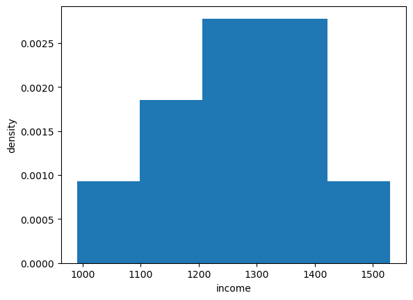
19.3.2.1. Histograms#
We can histogram the income distribution we just constructed as follows
fig, ax = plt.subplots()
ax.hist(x, bins=5, density=True, histtype='bar')
ax.set_xlabel('income')
ax.set_ylabel('density')
plt.show()
Let’s look at a distribution from real data.
In particular, we will look at the monthly return on Amazon shares between 2000/1/1 and 2024/1/1.
The monthly return is calculated as the percent change in the share price over each month.
So we will have one observation for each month.
df = yf.download('AMZN', '2000-1-1', '2024-1-1', interval='1mo')
prices = df['Close']
x_amazon = prices.pct_change()[1:] * 100
x_amazon.head()
The first observation is the monthly return (percent change) over January 2000, which was
x_amazon.iloc[0]
Ticker
AMZN    6.679568
Name: 2000-02-01 00:00:00, dtype: float64
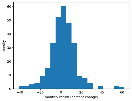
Let’s turn the return observations into an array and histogram it.
fig, ax = plt.subplots()
ax.hist(x_amazon, bins=20)
ax.set_xlabel('monthly return (percent change)')
ax.set_ylabel('density')
plt.show()
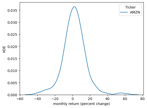
19.3.2.2. Kernel density estimates#
Kernel density estimates (KDE) provide a simple way to estimate and visualize the density of a distribution.
If you are not familiar with KDEs, you can think of them as a smoothed histogram.
Let’s have a look at a KDE formed from the Amazon return data.
fig, ax = plt.subplots()
sns.kdeplot(x_amazon, ax=ax)
ax.set_xlabel('monthly return (percent change)')
ax.set_ylabel('KDE')
plt.show()
The smoothness of the KDE is dependent on how we choose the bandwidth.
fig, ax = plt.subplots()
sns.kdeplot(x_amazon, ax=ax, bw_adjust=0.1, alpha=0.5, label="bw=0.1")
sns.kdeplot(x_amazon, ax=ax, bw_adjust=0.5, alpha=0.5, label="bw=0.5")
sns.kdeplot(x_amazon, ax=ax, bw_adjust=1, alpha=0.5, label="bw=1")
ax.set_xlabel('monthly return (percent change)')
ax.set_ylabel('KDE')
plt.legend()
plt.show()
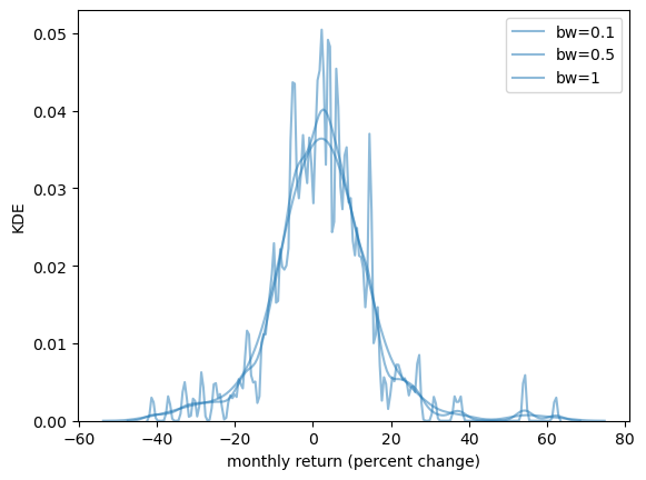
When we use a larger bandwidth, the KDE is smoother.
A suitable bandwidth is not too smooth (underfitting) or too wiggly (overfitting).
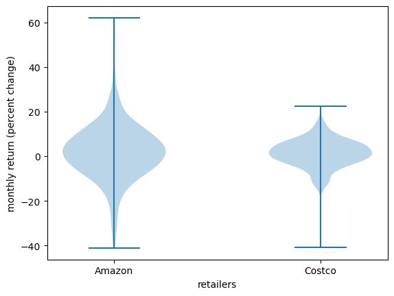
19.3.2.3. Violin plots#
Another way to display an observed distribution is via a violin plot.
fig, ax = plt.subplots()
ax.violinplot(x_amazon)
ax.set_ylabel('monthly return (percent change)')
ax.set_xlabel('KDE')
plt.show()
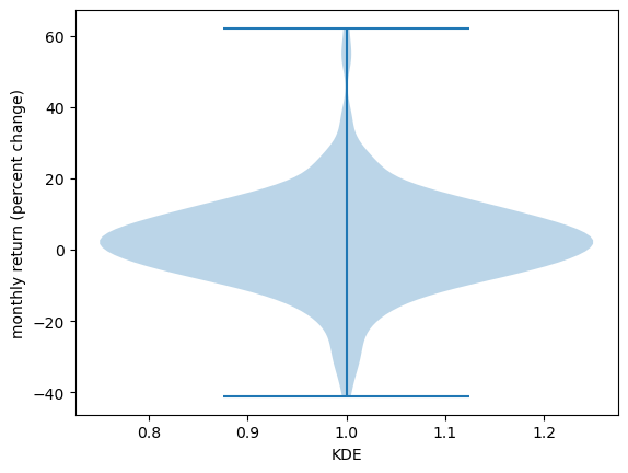
Violin plots are particularly useful when we want to compare different distributions.
For example, let’s compare the monthly returns on Amazon shares with the monthly return on Costco shares.
df = yf.download('COST', '2000-1-1', '2024-1-1', interval='1mo')
prices = df['Close']
x_costco = prices.pct_change()[1:] * 100
fig, ax = plt.subplots()
ax.violinplot([x_amazon['AMZN'], x_costco['COST']])
ax.set_ylabel('monthly return (percent change)')
ax.set_xlabel('retailers')

ax.set_xticks([1, 2])
ax.set_xticklabels(['Amazon', 'Costco'])
plt.show()
19.3.3. Connection to probability distributions#
Let’s discuss the connection between observed distributions and probability distributions.
Sometimes it’s helpful to imagine that an observed distribution is generated by a particular probability distribution.
For example, we might look at the returns from Amazon above and imagine that they were generated by a normal distribution.
(Even though this is not true, it might be a helpful way to think about the data.)
Here we match a normal distribution to the Amazon monthly returns by setting the sample mean to the mean of the normal distribution and the sample variance equal to the variance.
Then we plot the density and the histogram.
μ = x_amazon.mean()
σ_squared = x_amazon.var()
σ = np.sqrt(σ_squared)
u = scipy.stats.norm(μ, σ)
x_grid = np.linspace(-50, 65, 200)
fig, ax = plt.subplots()
ax.plot(x_grid, u.pdf(x_grid))
ax.hist(x_amazon, density=True, bins=40)
ax.set_xlabel('monthly return (percent change)')
ax.set_ylabel('density')
plt.show()
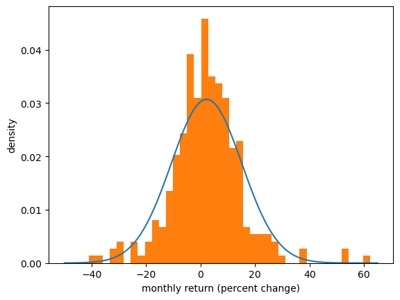
The match between the histogram and the density is not bad but also not very good.
One reason is that the normal distribution is not really a good fit for this observed data — we will discuss this point again when we talk about heavy tailed distributions.
Of course, if the data really is generated by the normal distribution, then the fit will be better.
Let’s see this in action
first we generate random draws from the normal distribution
then we histogram them and compare with the density.
μ, σ = 0, 1
u = scipy.stats.norm(μ, σ)
N = 2000  # Number of observations
x_draws = u.rvs(N)
x_grid = np.linspace(-4, 4, 200)
fig, ax = plt.subplots()
ax.plot(x_grid, u.pdf(x_grid))
ax.hist(x_draws, density=True, bins=40)
ax.set_xlabel('x')
ax.set_ylabel('density')
plt.show()
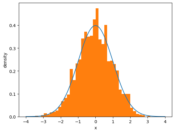
Note that if you keep increasing \(N\), which is the number of observations, the fit will get better and better.
This convergence is a version of the “law of large numbers”, which we will discuss later.