24. The Overlapping Generations Model

In this lecture we study the famous overlapping generations (OLG) model, which is used by policy makers and researchers to examine

• fiscal policy

• monetary policy

• long run growth

and many other topics.

The first rigorous version of the OLG model was developed by Paul Samuelson [Samuelson, 1958].

Our aim is to gain a good understanding of a simple version of the OLG model.

24.1. Overview

The dynamics of the OLG model are quite similar to those of the Solow-Swan growth model.

At the same time, the OLG model adds an important new feature: the choice of how much to save is endogenous.

To see why this is important, suppose, for example, that we are interested in predicting the effect of a new tax on long-run growth.

We could add a tax to the Solow-Swan model and look at the change in the steady state.

But this ignores the fact that households will change their savings and consumption behavior when they face the new tax rate.

Such changes can substantially alter the predictions of the model.

Hence, if we care about accurate predictions, we should model the decision problems of the agents.

In particular, households in the model should decide how much to save and how much to consume, given the environment that they face (technology, taxes, prices, etc.)

The OLG model takes up this challenge.

We will present a simple version of the OLG model that clarifies the decision problem of households and studies the implications for long run growth.

Let’s start with some imports.

import numpy as np
from scipy import optimize
from collections import namedtuple
import matplotlib.pyplot as plt

24.2. Environment

We assume that time is discrete, so that \(t=0, 1, \ldots\),

An individual born at time \(t\) lives for two periods, \(t\) and \(t + 1\).

We call an agent

• “young” during the first period of their lives and

• “old” during the second period of their lives.

Young agents work, supplying labor and earning labor income.

They also decide how much to save.

Old agents do not work, so all income is financial.

Their financial income is from interest on their savings from wage income, which is then combined with the labor of the new young generation at \(t+1\).

The wage and interest rates are determined in equilibrium by supply and demand.

To make the algebra slightly easier, we are going to assume a constant population size.

We normalize the constant population size in each period to 1.

We also suppose that each agent supplies one “unit” of labor hours, so total labor supply is 1.

24.3. Supply of capital

First let’s consider the household side.

24.3.1. Consumer’s problem

Suppose that utility for individuals born at time \(t\) takes the form

(24.1)\[ U_t = u(c_t) + \beta u(c_{t+1})\]

Here

• \(u: \mathbb R_+ \to \mathbb R\) is called the “flow” utility function

• \(\beta \in (0, 1)\) is the discount factor

• \(c_t\) is time \(t\) consumption of the individual born at time \(t\)

• \(c_{t+1}\) is time \(t+1\) consumption of the same individual

We assume that \(u\) is strictly increasing.

Savings behavior is determined by the optimization problem

(24.2)\[ \max_{c_t, c_{t+1}} \, \left \{ u(c_t) + \beta u(c_{t+1}) \right \} \]

subject to

\[ c_t + s_t \le w_t \quad \text{and} \quad c_{t+1} \le R_{t+1} s_t \]

Here

• \(s_t\) is savings by an individual born at time \(t\)

• \(w_t\) is the wage rate at time \(t\)

• \(R_{t+1}\) is the interest rate on savings invested at time \(t\), paid at time \(t+1\)

Since \(u\) is strictly increasing, both of these constraints will hold as equalities at the maximum.

Using this fact and substituting \(s_t\) from the first constraint into the second we get \(c_{t+1} = R_{t+1}(w_t - c_t)\).

The first-order condition for a maximum can be obtained by plugging \(c_{t+1}\) into the objective function, taking the derivative with respect to \(c_t\), and setting it to zero.

This leads to the Euler equation of the OLG model, which is

(24.3)\[ u'(c_t) = \beta R_{t+1} u'( R_{t+1} (w_t - c_t))\]

From the first constraint we get \(c_t = w_t - s_t\), so the Euler equation can also be expressed as

(24.4)\[ u'(w_t - s_t) = \beta R_{t+1} u'( R_{t+1} s_t)\]

Suppose that, for each \(w_t\) and \(R_{t+1}\), there is exactly one \(s_t\) that solves (24.4).

Then savings can be written as a fixed function of \(w_t\) and \(R_{t+1}\).

We write this as

(24.5)\[ s_t = s(w_t, R_{t+1})\]

The precise form of the function \(s\) will depend on the choice of flow utility function \(u\).

Together, \(w_t\) and \(R_{t+1}\) represent the prices in the economy (price of labor and rental rate of capital).

Thus, (24.5) states the quantity of savings given prices.

24.3.2. Example: log preferences

In the special case \(u(c) = \log c\), the Euler equation simplifies to \(s_t= \beta (w_t - s_t)\).

Solving for saving, we get

(24.6)\[ s_t = s(w_t, R_{t+1}) = \frac{\beta}{1+\beta} w_t\]

In this special case, savings does not depend on the interest rate.

24.3.3. Savings and investment

Since the population size is normalized to 1, \(s_t\) is also total savings in the economy at time \(t\).

In our closed economy, there is no foreign investment, so net savings equals total investment, which can be understood as supply of capital to firms.

In the next section we investigate demand for capital.

Equating supply and demand will allow us to determine equilibrium in the OLG economy.

24.4. Demand for capital

First we describe the firm problem and then we write down an equation describing demand for capital given prices.

24.4.1. Firm’s problem

For each integer \(t \geq 0\), output \(y_t\) in period \(t\) is given by the Cobb-Douglas production function

(24.7)\[ y_t = k_t^{\alpha} \ell_t^{1-\alpha}\]

Here \(k_t\) is capital, \(\ell_t\) is labor, and \(\alpha\) is a parameter (sometimes called the “output elasticity of capital”).

The profit maximization problem of the firm is

(24.8)\[ \max_{k_t, \ell_t} \{ k^{\alpha}_t \ell_t^{1-\alpha} - R_t k_t - \ell_t w_t \}\]

The first-order conditions are obtained by taking the derivative of the objective function with respect to capital and labor respectively and setting them to zero:

\[ (1-\alpha)(k_t / \ell_t)^{\alpha} = w_t \quad \text{and} \quad \alpha (k_t / \ell_t)^{\alpha - 1} = R_t\]

24.4.2. Demand

Using our assumption \(\ell_t = 1\) allows us to write

(24.9)\[ w_t = (1-\alpha)k_t^\alpha \]

and

(24.10)\[ R_t = \alpha k_t^{\alpha - 1} \]

Rearranging (24.10) gives the aggregate demand for capital at time \(t+1\)

(24.11)\[ k^d (R_{t+1}) := \left (\frac{\alpha}{R_{t+1}} \right )^{1/(1-\alpha)}\]

In Python code this is

def capital_demand(R, α):
    return (α/R)**(1/(1-α)) 

def capital_supply(R, β, w):
    R = np.ones_like(R)
    return R * (β / (1 + β)) * w

The next figure plots the supply of capital, as in (24.6), as well as the demand for capital, as in (24.11), as functions of the interest rate \(R_{t+1}\).

(For the special case of log utility, supply does not depend on the interest rate, so we have a constant function.)

R_vals = np.linspace(0.3, 1)
α, β = 0.5, 0.9
w = 2.0

fig, ax = plt.subplots()

ax.plot(R_vals, capital_demand(R_vals, α), 
        label="aggregate demand")
ax.plot(R_vals, capital_supply(R_vals, β, w), 
        label="aggregate supply")

ax.set_xlabel("$R_{t+1}$")
ax.set_ylabel("$k_{t+1}$")
ax.legend()
plt.show()

24.5. Equilibrium

In this section we derive equilibrium conditions and investigate an example.

24.5.1. Equilibrium conditions

In equilibrium, savings at time \(t\) equals investment at time \(t\), which equals capital supply at time \(t+1\).

Equilibrium is computed by equating these quantities, setting

(24.12)\[ s(w_t, R_{t+1}) = k^d(R_{t+1}) = \left (\frac{\alpha}{R_{t+1}} \right )^{1/(1-\alpha)}\]

In principle, we can now solve for the equilibrium price \(R_{t+1}\) given \(w_t\).

(In practice, we first need to specify the function \(u\) and hence \(s\).)

When we solve this equation, which concerns time \(t+1\) outcomes, time \(t\) quantities are already determined, so we can treat \(w_t\) as a constant.

From equilibrium \(R_{t+1}\) and (24.11), we can obtain the equilibrium quantity \(k_{t+1}\).

24.5.2. Example: log utility

In the case of log utility, we can use (24.12) and (24.6) to obtain

(24.13)\[ \frac{\beta}{1+\beta} w_t = \left( \frac{\alpha}{R_{t+1}} \right)^{1/(1-\alpha)}\]

Solving for the equilibrium interest rate gives

(24.14)\[ R_{t+1} = \alpha \left( \frac{\beta}{1+\beta} w_t \right)^{\alpha-1}\]

In Python we can compute this via

def equilibrium_R_log_utility(α, β, w):
    R = α * ( (β * w) / (1 + β))**(α - 1)
    return R

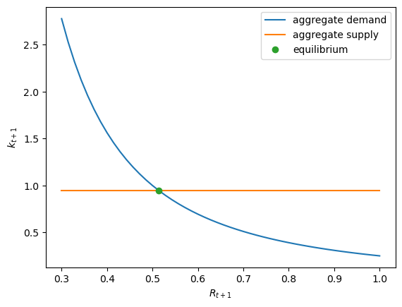
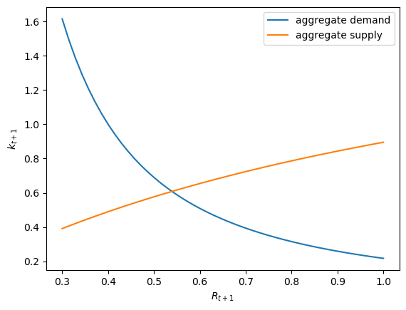
In the case of log utility, since capital supply does not depend on the interest rate, the equilibrium quantity is fixed by supply.

That is,

(24.15)\[ k_{t+1} = s(w_t, R_{t+1}) = \frac{\beta }{1+\beta} w_t\]

Let’s redo our plot above but now inserting the equilibrium quantity and price.

R_vals = np.linspace(0.3, 1)
α, β = 0.5, 0.9
w = 2.0

fig, ax = plt.subplots()

ax.plot(R_vals, capital_demand(R_vals, α), 
        label="aggregate demand")
ax.plot(R_vals, capital_supply(R_vals, β, w), 
        label="aggregate supply")

R_e = equilibrium_R_log_utility(α, β, w)
k_e = (β / (1 + β)) * w

ax.plot(R_e, k_e, 'go', ms=6, alpha=0.6)

ax.annotate(r'equilibrium',
             xy=(R_e, k_e),
             xycoords='data',
             xytext=(0, 60),
             textcoords='offset points',
             fontsize=12,
             arrowprops=dict(arrowstyle="->"))

ax.set_xlabel("$R_{t+1}$")
ax.set_ylabel("$k_{t+1}$")
ax.legend()
plt.show()

24.6. Dynamics

In this section we discuss dynamics.

For now we will focus on the case of log utility, so that the equilibrium is determined by (24.15).

24.6.1. Evolution of capital

The discussion above shows how equilibrium \(k_{t+1}\) is obtained given \(w_t\).

From (24.9) we can translate this into \(k_{t+1}\) as a function of \(k_t\)

In particular, since \(w_t = (1-\alpha)k_t^\alpha\), we have

(24.16)\[ k_{t+1} = \frac{\beta}{1+\beta} (1-\alpha)(k_t)^{\alpha}\]

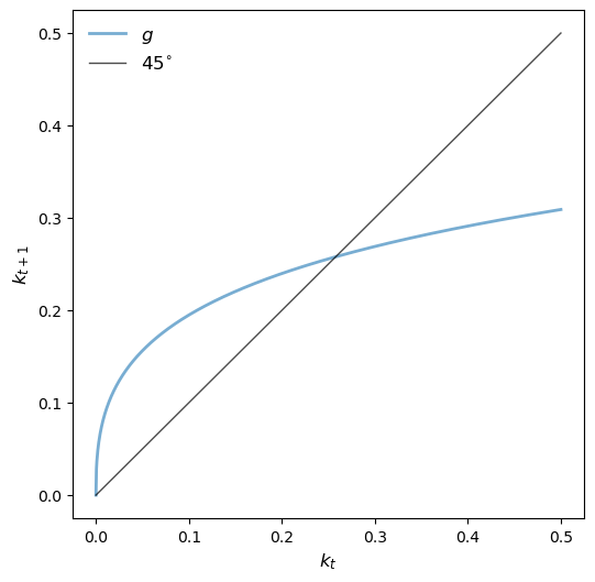
If we iterate on this equation, we get a sequence for capital stock.

Let’s plot the 45 degree diagram of these dynamics, which we write as

\[ k_{t+1} = g(k_t) \quad \text{where } g(k) := \frac{\beta}{1+\beta} (1-\alpha)(k)^{\alpha} \]

def k_update(k, α, β):
    return β * (1 - α) * k**α /  (1 + β)

α, β = 0.5, 0.9
kmin, kmax = 0, 0.1
x = 1000
k_grid = np.linspace(kmin, kmax, x)
k_grid_next = np.empty_like(k_grid)

for i in range(x):
    k_grid_next[i] = k_update(k_grid[i], α, β)

fig, ax = plt.subplots(figsize=(6, 6))

ymin, ymax = np.min(k_grid_next), np.max(k_grid_next)

ax.plot(k_grid, k_grid_next,  lw=2, alpha=0.6, label='$g$')
ax.plot(k_grid, k_grid, 'k-', lw=1, alpha=0.7, label='$45^{\circ}$')


ax.legend(loc='upper left', frameon=False, fontsize=12)
ax.set_xlabel('$k_t$', fontsize=12)
ax.set_ylabel('$k_{t+1}$', fontsize=12)

plt.show()

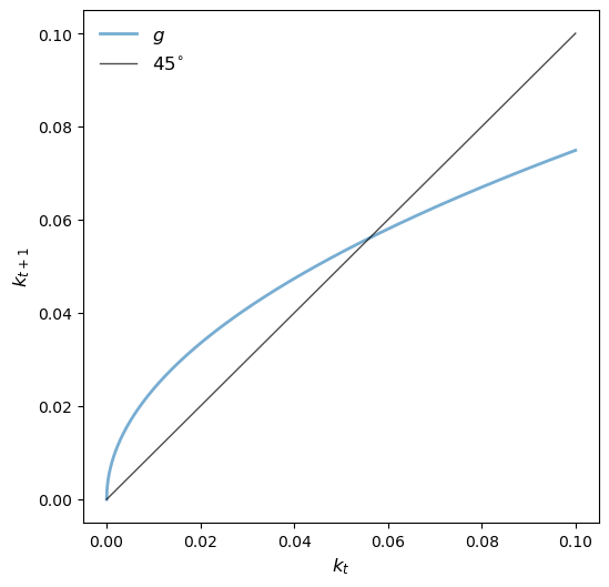
24.6.2. Steady state (log case)

The diagram shows that the model has a unique positive steady state, which we denote by \(k^*\).

We can solve for \(k^*\) by setting \(k^* = g(k^*)\), or

(24.17)\[ k^* = \frac{\beta (1-\alpha) (k^*)^{\alpha}}{(1+\beta)}\]

Solving this equation yields

(24.18)\[ k^* = \left (\frac{\beta (1-\alpha)}{1+\beta} \right )^{1/(1-\alpha)}\]

We can get the steady state interest rate from (24.10), which yields

\[ R^* = \alpha (k^*)^{\alpha - 1} = \frac{\alpha}{1 - \alpha} \frac{1 + \beta}{\beta} \]

In Python we have

k_star = ((β * (1 - α))/(1 + β))**(1/(1-α))
R_star = (α/(1 - α)) * ((1 + β) / β)

24.6.3. Time series

The 45 degree diagram above shows that time series of capital with positive initial conditions converge to this steady state.

Let’s plot some time series that visualize this.

ts_length = 25
k_series = np.empty(ts_length)
k_series[0] = 0.02
for t in range(ts_length - 1):
    k_series[t+1] = k_update(k_series[t], α, β)

fig, ax = plt.subplots()
ax.plot(k_series, label="capital series")
ax.plot(range(ts_length), np.full(ts_length, k_star), 'k--', label="$k^*$")
ax.set_ylim(0, 0.1)
ax.set_ylabel("capital")
ax.set_xlabel("$t$")
ax.legend()
plt.show()

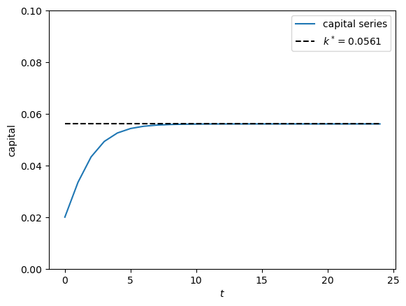
If you experiment with different positive initial conditions, you will see that the series always converges to \(k^*\).

Below we also plot the gross interest rate over time.

R_series = α * k_series**(α - 1)

fig, ax = plt.subplots()
ax.plot(R_series, label="gross interest rate")
ax.plot(range(ts_length), np.full(ts_length, R_star), 'k--', label="$R^*$")
ax.set_ylim(0, 4)
ax.set_xlabel("$t$")
ax.legend()
plt.show()

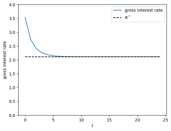
The interest rate reflects the marginal product of capital, which is high when capital stock is low.

24.7. CRRA preferences

Previously, in our examples, we looked at the case of log utility.

Log utility is a rather special case.

In this section, we are going to assume that \(u(c) = \frac{ c^{1- \gamma}-1}{1-\gamma}\), where \(\gamma >0, \gamma\neq 1\).

This function is called the CRRA utility function.

In other respects, the model is the same.

Below we define the utility function in Python and construct a namedtuple to store the parameters.

def crra(c, γ):
    return c**(1 - γ) / (1 - γ)

Model = namedtuple('Model', ['α',        # Cobb-Douglas parameter
                             'β',        # discount factor
                             'γ']        # parameter in CRRA utility
                   )

def create_olg_model(α=0.4, β=0.9, γ=0.5):
    return Model(α=α, β=β, γ=γ)

Let’s also redefine the capital demand function to work with this namedtuple.

def capital_demand(R, model):
    return (α/R)**(1/(1-model.α)) 

24.7.1. Supply

For households, the Euler equation becomes

(24.19)\[ (w_t - s_t)^{-\gamma} = \beta R^{1-\gamma}_{t+1} (s_t)^{-\gamma}\]

Solving for savings, we have

(24.20)\[ s_t = s(w_t, R_{t+1}) = w_t \left [ 1 + \beta^{-1/\gamma} R_{t+1}^{(\gamma-1)/\gamma} \right ]^{-1}\]

Notice how, unlike the log case, savings now depends on the interest rate.

def savings_crra(w, R, model):
    α, β, γ = model
    return w / (1 + β**(-1/γ) * R**((γ-1)/γ)) 

R_vals = np.linspace(0.3, 1)
model = create_olg_model()
w = 2.0

fig, ax = plt.subplots()

ax.plot(R_vals, capital_demand(R_vals, model), 
        label="aggregate demand")
ax.plot(R_vals, savings_crra(w, R_vals, model), 
        label="aggregate supply")

ax.set_xlabel("$R_{t+1}$")
ax.set_ylabel("$k_{t+1}$")
ax.legend()
plt.show()

24.7.2. Equilibrium

Equating aggregate demand for capital (see (24.11)) with our new aggregate supply function yields equilibrium capital.

Thus, we set

(24.21)\[ w_t \left [ 1 + \beta^{-1/\gamma} R_{t+1}^{(\gamma-1)/\gamma} \right ]^{-1} = \left (\frac{R_{t+1}}{\alpha} \right )^{1/(\alpha - 1)}\]

This expression is quite complex and we cannot solve for \(R_{t+1}\) analytically.

Combining (24.10) and (24.21) yields

(24.22)\[ k_{t+1} = \left [ 1 + \beta^{-1/\gamma} (\alpha k^{\alpha - 1}_{t+1})^{(\gamma-1)/\gamma} \right ]^{-1} (1-\alpha)(k_t)^{\alpha}\]

Again, with this equation and \(k_t\) as given, we cannot solve for \(k_{t+1}\) by pencil and paper.

In the exercise below, you will be asked to solve these equations numerically.

24.8. Exercises

Exercise 24.1

Solve for the dynamics of equilibrium capital stock in the CRRA case numerically using (24.22).

Visualize the dynamics using a 45 degree diagram.

Solution to Exercise 24.1

To solve for \(k_{t+1}\) given \(k_t\) we use Newton’s method.

Let

(24.23)\[ f(k_{t+1}, k_t) = k_{t+1} \left[ 1 + \beta^{-1/\gamma} \left ( \alpha k^{\alpha-1}_{t+1} \right )^{(\gamma-1)/\gamma} \right] - (1-\alpha) k^{\alpha}_t =0\]

If \(k_t\) is given then \(f\) is a function of unknown \(k_{t+1}\).

Then we can use scipy.optimize.newton to solve \(f(k_{t+1}, k_t)=0\) for \(k_{t+1}\).

First let’s define \(f\).

def f(k_prime, k, model):
    α, β, γ = model.α, model.β, model.γ
    z = (1 - α) * k**α
    a = α**(1-1/γ)
    b = k_prime**((α * γ - α + 1) / γ)
    p = k_prime + k_prime * β**(-1/γ) * a * b
    return p - z

Now let’s define a function that finds the value of \(k_{t+1}\).

def k_update(k, model):
    return optimize.newton(lambda k_prime: f(k_prime, k, model), 0.1)

Finally, here is the 45 degree diagram.

kmin, kmax = 0, 0.5
x = 1000
k_grid = np.linspace(kmin, kmax, x)
k_grid_next = np.empty_like(k_grid)

for i in range(x):
    k_grid_next[i] = k_update(k_grid[i], model)

fig, ax = plt.subplots(figsize=(6, 6))

ymin, ymax = np.min(k_grid_next), np.max(k_grid_next)

ax.plot(k_grid, k_grid_next,  lw=2, alpha=0.6, label='$g$')
ax.plot(k_grid, k_grid, 'k-', lw=1, alpha=0.7, label='$45^{\circ}$')


ax.legend(loc='upper left', frameon=False, fontsize=12)
ax.set_xlabel('$k_t$', fontsize=12)
ax.set_ylabel('$k_{t+1}$', fontsize=12)

plt.show()

Exercise 24.2

The 45 degree diagram from the last exercise shows that there is a unique positive steady state.

The positive steady state can be obtained by setting \(k_{t+1} = k_t = k^*\) in (24.22), which yields

\[ k^* = \frac{(1-\alpha)(k^*)^{\alpha}} {1 + \beta^{-1/\gamma} (\alpha (k^*)^{\alpha-1})^{(\gamma-1)/\gamma}} \]

Unlike the log preference case, the CRRA utility steady state \(k^*\) cannot be obtained analytically.

Instead, we solve for \(k^*\) using Newton’s method.

Solution to Exercise 24.2

We introduce a function \(h\) such that positive steady state is the root of \(h\).

(24.24)\[ h(k^*) = k^* \left [ 1 + \beta^{-1/\gamma} (\alpha (k^*)^{\alpha-1})^{(\gamma-1)/\gamma} \right ] - (1-\alpha)(k^*)^{\alpha}\]

Here it is in Python

def h(k_star, model):
    α, β, γ = model.α, model.β, model.γ
    z = (1 - α) * k_star**α
    R1 = α ** (1-1/γ)
    R2 = k_star**((α * γ - α + 1) / γ)
    p = k_star + k_star * β**(-1/γ) * R1 * R2
    return p - z

Let’s apply Newton’s method to find the root:

k_star = optimize.newton(h, 0.2, args=(model,))
print(f"k_star = {k_star}")

k_star = 0.25788950250843484

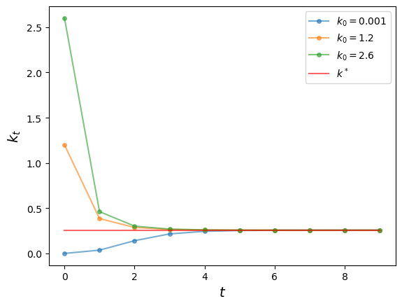
Exercise 24.3

Generate three time paths for capital, from three distinct initial conditions, under the parameterization listed above.

Use initial conditions for \(k_0\) of \(0.001, 1.2, 2.6\) and time series length 10.

Solution to Exercise 24.3

Let’s define the constants and three distinct intital conditions

ts_length = 10
k0 = np.array([0.001, 1.2, 2.6])

def simulate_ts(model, k0_values, ts_length):

    fig, ax = plt.subplots()

    ts = np.zeros(ts_length)

    # simulate and plot time series
    for k_init in k0_values:
        ts[0] = k_init
        for t in range(1, ts_length):
            ts[t] = k_update(ts[t-1], model)
        ax.plot(np.arange(ts_length), ts, '-o', ms=4, alpha=0.6,
                label=r'$k_0=%g$' %k_init)
    ax.plot(np.arange(ts_length), np.full(ts_length, k_star),
            alpha=0.6, color='red', label=r'$k^*$')
    ax.legend(fontsize=10)

    ax.set_xlabel(r'$t$', fontsize=14)
    ax.set_ylabel(r'$k_t$', fontsize=14)

    plt.show()

simulate_ts(model, k0, ts_length)