14. Equalizing Difference Model#
14.1. Overview#
This lecture presents a model of the college-high-school wage gap in which the “time to build” a college graduate plays a key role.
Milton Friedman invented the model to study whether differences in earnings of US dentists and doctors were outcomes of competitive labor markets or whether they reflected entry barriers imposed by governments working in conjunction with doctors’ professional organizations.
Chapter 4 of Jennifer Burns [Burns, 2023] describes Milton Friedman’s joint work with Simon Kuznets that eventually led to the publication of [Kuznets and Friedman, 1939] and [Friedman and Kuznets, 1945].
To map Friedman’s application into our model, think of our high school students as Friedman’s dentists and our college graduates as Friedman’s doctors.
Our presentation is “incomplete” in the sense that it is based on a single equation that would be part of set equilibrium conditions of a more fully articulated model.
This ‘‘equalizing difference’’ equation determines a college-high-school wage ratio that equalizes present values of a high school educated worker and a college educated worker.
The idea is that lifetime earnings somehow adjust to make a new high school worker indifferent between going to college and not going to college but instead going to work immediately.
(The job of the “other equations” in a more complete model would be to describe what adjusts to bring about this outcome.)
Our model is just one example of an “equalizing difference” theory of relative wage rates, a class of theories dating back at least to Adam Smith’s Wealth of Nations [Smith, 2010].
For most of this lecture, the only mathematical tools that we’ll use are from linear algebra, in particular, matrix multiplication and matrix inversion.
However, near the end of the lecture, we’ll use calculus just in case readers want to see how computing partial derivatives could let us present some findings more concisely.
And doing that will let illustrate how good Python is at doing calculus!
But if you don’t know calculus, our tools from linear algebra are certainly enough.
As usual, we’ll start by importing some Python modules.
import numpy as np
import matplotlib.pyplot as plt
from collections import namedtuple
from sympy import Symbol, Lambda, symbols
14.2. The indifference condition#
The key idea is that the entry level college wage premium has to adjust to make a representative worker indifferent between going to college and not going to college.
Let
\(R > 1\) be the gross rate of return on a one-period bond
\(t = 0, 1, 2, \ldots T\) denote the years that a person either works or attends college
\(0\) denote the first period after high school that a person can work if he does not go to college
\(T\) denote the last period that a person works
\(w_t^h\) be the wage at time \(t\) of a high school graduate
\(w_t^c\) be the wage at time \(t\) of a college graduate
\(\gamma_h > 1\) be the (gross) rate of growth of wages of a high school graduate, so that \( w_t^h = w_0^h \gamma_h^t\)
\(\gamma_c > 1\) be the (gross) rate of growth of wages of a college graduate, so that \( w_t^c = w_0^c \gamma_c^t\)
\(D\) be the upfront monetary costs of going to college
We now compute present values that a new high school graduate earns if
he goes to work immediately and earns wages paid to someone without a college education
he goes to college for four years and after graduating earns wages paid to a college graduate
14.2.1. Present value of a high school educated worker#
If someone goes to work immediately after high school and works for the \(T+1\) years \(t=0, 1, 2, \ldots, T\), she earns present value
where
The present value \(h_0\) is the “human wealth” at the beginning of time \(0\) of someone who chooses not to attend college but instead to go to work immediately at the wage of a high school graduate.
14.2.2. Present value of a college-bound new high school graduate#
If someone goes to college for the four years \(t=0, 1, 2, 3\) during which she earns \(0\), but then goes to work immediately after college and works for the \(T-3\) years \(t=4, 5, \ldots ,T\), she earns present value
where
The present value \(c_0\) is the “human wealth” at the beginning of time \(0\) of someone who chooses to attend college for four years and then start to work at time \(t=4\) at the wage of a college graduate.
Assume that college tuition plus four years of room and board amount to \(D\) and must be paid at time \(0\).
So net of monetary cost of college, the present value of attending college as of the first period after high school is
We now formulate a pure equalizing difference model of the initial college-high school wage gap \(\phi\) that verifies
We suppose that \(R, \gamma_h, \gamma_c, T\) and also \(w_0^h\) are fixed parameters.
We start by noting that the pure equalizing difference model asserts that the college-high-school wage gap \(\phi\) solves an “equalizing” equation that sets the present value not going to college equal to the present value of going to college:
or
This “indifference condition” is the heart of the model.
Solving equation (14.1) for the college wage premium \(\phi\) we obtain
In a free college special case \(D =0\).
Here the only cost of going to college is the forgone earnings from being a high school educated worker.
In that case,
In the next section we’ll write Python code to compute \(\phi\) and plot it as a function of its determinants.
14.3. Computations#
We can have some fun with examples that tweak various parameters, prominently including \(\gamma_h, \gamma_c, R\).
Now let’s write some Python code to compute \(\phi\) and plot it as a function of some of its determinants.
# Define the namedtuple for the equalizing difference model
EqDiffModel = namedtuple('EqDiffModel', 'R T γ_h γ_c w_h0 D')

def create_edm(R=1.05,   # gross rate of return
               T=40,     # time horizon
               γ_h=1.01, # high-school wage growth
               γ_c=1.01, # college wage growth
               w_h0=1,   # initial wage (high school)
               D=10,     # cost for college
              ):

    return EqDiffModel(R, T, γ_h, γ_c, w_h0, D)

def compute_gap(model):
    R, T, γ_h, γ_c, w_h0, D = model

    A_h = (1 - (γ_h/R)**(T+1)) / (1 - γ_h/R)
    A_c = (1 - (γ_c/R)**(T-3)) / (1 - γ_c/R) * (γ_c/R)**4
    ϕ = A_h / A_c + D / (w_h0 * A_c)

    return ϕ
Using vectorization instead of loops, we build some functions to help do comparative statics .
For a given instance of the class, we want to recompute \(\phi\) when one parameter changes and others remain fixed.
Let’s do an example.
ex1 = create_edm()
gap1 = compute_gap(ex1)

gap1
1.8041412724969135
Let’s not charge for college and recompute \(\phi\).
The initial college wage premium should go down.
# free college
ex2 = create_edm(D=0)
gap2 = compute_gap(ex2)
gap2
1.2204649517903732
Let us construct some graphs that show us how the initial college-high-school wage ratio \(\phi\) would change if one of its determinants were to change.
Let’s start with the gross interest rate \(R\).
R_arr = np.linspace(1, 1.2, 50)
models = [create_edm(R=r) for r in R_arr]
gaps = [compute_gap(model) for model in models]

plt.plot(R_arr, gaps)
plt.xlabel(r'$R$')
plt.ylabel(r'wage gap')
plt.show()
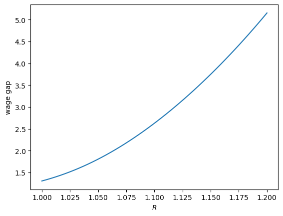
Evidently, the initial wage ratio \(\phi\) must rise to compensate a prospective high school student for waiting to start receiving income – remember that while she is earning nothing in years \(t=0, 1, 2, 3\), the high school worker is earning a salary.
Not let’s study what happens to the initial wage ratio \(\phi\) if the rate of growth of college wages rises, holding constant other determinants of \(\phi\).
γc_arr = np.linspace(1, 1.2, 50)
models = [create_edm(γ_c=γ_c) for γ_c in γc_arr]
gaps = [compute_gap(model) for model in models]

plt.plot(γc_arr, gaps)
plt.xlabel(r'$\gamma_c$')
plt.ylabel(r'wage gap')
plt.show()
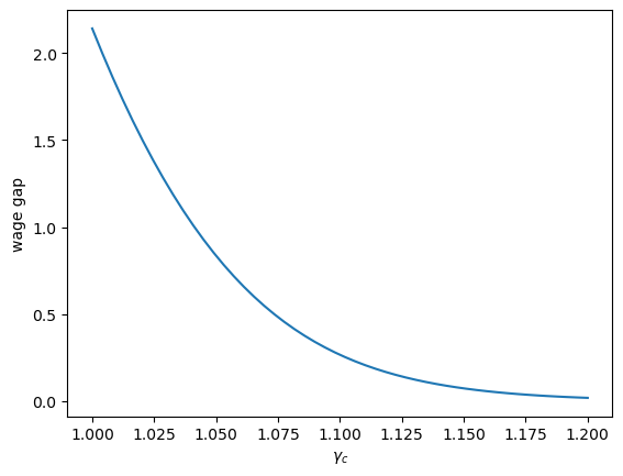
Notice how the initial wage gap falls when the rate of growth \(\gamma_c\) of college wages rises.
The wage gap falls to “equalize” the present values of the two types of career, one as a high school worker, the other as a college worker.
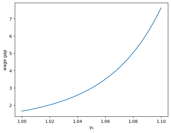
Can you guess what happens to the initial wage ratio \(\phi\) when next we vary the rate of growth of high school wages, holding all other determinants of \(\phi\) constant?
The following graph shows what happens.
γh_arr = np.linspace(1, 1.1, 50)
models = [create_edm(γ_h=γ_h) for γ_h in γh_arr]
gaps = [compute_gap(model) for model in models]

plt.plot(γh_arr, gaps)
plt.xlabel(r'$\gamma_h$')
plt.ylabel(r'wage gap')
plt.show()
14.4. Entrepreneur-worker interpretation#
We can add a parameter and reinterpret variables to get a model of entrepreneurs versus workers.
We now let \(h\) be the present value of a “worker”.
We define the present value of an entrepreneur to be
where \(\pi \in (0,1) \) is the probability that an entrepreneur’s “project” succeeds.
For our model of workers and firms, we’ll interpret \(D\) as the cost of becoming an entrepreneur.
This cost might include costs of hiring workers, office space, and lawyers.
What we used to call the college, high school wage gap \(\phi\) now becomes the ratio of a successful entrepreneur’s earnings to a worker’s earnings.
We’ll find that as \(\pi\) decreases, \(\phi\) increases, indicating that the riskier it is to be an entrepreneur, the higher must be the reward for a successful project.
Now let’s adopt the entrepreneur-worker interpretation of our model
# Define a model of entrepreneur-worker interpretation
EqDiffModel = namedtuple('EqDiffModel', 'R T γ_h γ_c w_h0 D π')

def create_edm_π(R=1.05,   # gross rate of return
                 T=40,     # time horizon
                 γ_h=1.01, # high-school wage growth
                 γ_c=1.01, # college wage growth
                 w_h0=1,   # initial wage (high school)
                 D=10,     # cost for college
                 π=0       # chance of business success
              ):

    return EqDiffModel(R, T, γ_h, γ_c, w_h0, D, π)


def compute_gap(model):
    R, T, γ_h, γ_c, w_h0, D, π = model

    A_h = (1 - (γ_h/R)**(T+1)) / (1 - γ_h/R)
    A_c = (1 - (γ_c/R)**(T-3)) / (1 - γ_c/R) * (γ_c/R)**4

    # Incorprate chance of success
    A_c = π * A_c

    ϕ = A_h / A_c + D / (w_h0 * A_c)
    return ϕ
If the probability that a new business succeeds is \(0.2\), let’s compute the initial wage premium for successful entrepreneurs.
ex3 = create_edm_π(π=0.2)
gap3 = compute_gap(ex3)

gap3
9.020706362484567
Now let’s study how the initial wage premium for successful entrepreneurs depend on the success probability.
π_arr = np.linspace(0.2, 1, 50)
models = [create_edm_π(π=π) for π in π_arr]
gaps = [compute_gap(model) for model in models]

plt.plot(π_arr, gaps)
plt.ylabel(r'wage gap')
plt.xlabel(r'$\pi$')
plt.show()
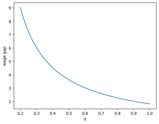
Does the graph make sense to you?
14.5. An application of calculus#
So far, we have used only linear algebra and it has been a good enough tool for us to figure out how our model works.
However, someone who knows calculus might want us just to take partial derivatives.
We’ll do that now.
A reader who doesn’t know calculus could read no further and feel confident that applying linear algebra has taught us the main properties of the model.
But for a reader interested in how we can get Python to do all the hard work involved in computing partial derivatives, we’ll say a few things about that now.
We’ll use the Python module ‘sympy’ to compute partial derivatives of \(\phi\) with respect to the parameters that determine it.
Define symbols
γ_h, γ_c, w_h0, D = symbols(r'\gamma_h, \gamma_c, w_0^h, D', real=True)
R, T = Symbol('R', real=True), Symbol('T', integer=True)
Define function \(A_h\)
A_h = Lambda((γ_h, R, T), (1 - (γ_h/R)**(T+1)) / (1 - γ_h/R))
A_h
Define function \(A_c\)
A_c = Lambda((γ_c, R, T), (1 - (γ_c/R)**(T-3)) / (1 - γ_c/R) * (γ_c/R)**4)
A_c
Now, define \(\phi\)
ϕ = Lambda((D, γ_h, γ_c, R, T, w_h0), A_h(γ_h, R, T)/A_c(γ_c, R, T) + D/(w_h0*A_c(γ_c, R, T)))
ϕ
We begin by setting default parameter values.
R_value = 1.05
T_value = 40
γ_h_value, γ_c_value = 1.01, 1.01
w_h0_value = 1
D_value = 10
Now let’s compute \(\frac{\partial \phi}{\partial D}\) and then evaluate it at the default values
ϕ_D = ϕ(D, γ_h, γ_c, R, T, w_h0).diff(D)
ϕ_D
# Numerical value at default parameters
ϕ_D_func = Lambda((D, γ_h, γ_c, R, T, w_h0), ϕ_D)
ϕ_D_func(D_value, γ_h_value, γ_c_value, R_value, T_value, w_h0_value)
Thus, as with our earlier graph, we find that raising \(R\) increases the initial college wage premium \(\phi\).
Compute \(\frac{\partial \phi}{\partial T}\) and evaluate it at default parameters
ϕ_T = ϕ(D, γ_h, γ_c, R, T, w_h0).diff(T)
ϕ_T
# Numerical value at default parameters
ϕ_T_func = Lambda((D, γ_h, γ_c, R, T, w_h0), ϕ_T)
ϕ_T_func(D_value, γ_h_value, γ_c_value, R_value, T_value, w_h0_value)
We find that raising \(T\) decreases the initial college wage premium \(\phi\).
This is because college graduates now have longer career lengths to “pay off” the time and other costs they paid to go to college
Let’s compute \(\frac{\partial \phi}{\partial γ_h}\) and evaluate it at default parameters.
ϕ_γ_h = ϕ(D, γ_h, γ_c, R, T, w_h0).diff(γ_h)
ϕ_γ_h
# Numerical value at default parameters
ϕ_γ_h_func = Lambda((D, γ_h, γ_c, R, T, w_h0), ϕ_γ_h)
ϕ_γ_h_func(D_value, γ_h_value, γ_c_value, R_value, T_value, w_h0_value)
We find that raising \(\gamma_h\) increases the initial college wage premium \(\phi\), in line with our earlier graphical analysis.
Compute \(\frac{\partial \phi}{\partial γ_c}\) and evaluate it numerically at default parameter values
ϕ_γ_c = ϕ(D, γ_h, γ_c, R, T, w_h0).diff(γ_c)
ϕ_γ_c
# Numerical value at default parameters
ϕ_γ_c_func = Lambda((D, γ_h, γ_c, R, T, w_h0), ϕ_γ_c)
ϕ_γ_c_func(D_value, γ_h_value, γ_c_value, R_value, T_value, w_h0_value)
We find that raising \(\gamma_c\) decreases the initial college wage premium \(\phi\), in line with our earlier graphical analysis.
Let’s compute \(\frac{\partial \phi}{\partial R}\) and evaluate it numerically at default parameter values
ϕ_R = ϕ(D, γ_h, γ_c, R, T, w_h0).diff(R)
ϕ_R
# Numerical value at default parameters
ϕ_R_func = Lambda((D, γ_h, γ_c, R, T, w_h0), ϕ_R)
ϕ_R_func(D_value, γ_h_value, γ_c_value, R_value, T_value, w_h0_value)
We find that raising the gross interest rate \(R\) increases the initial college wage premium \(\phi\), in line with our earlier graphical analysis.
14.6. Exercises#
Exercise 14.1
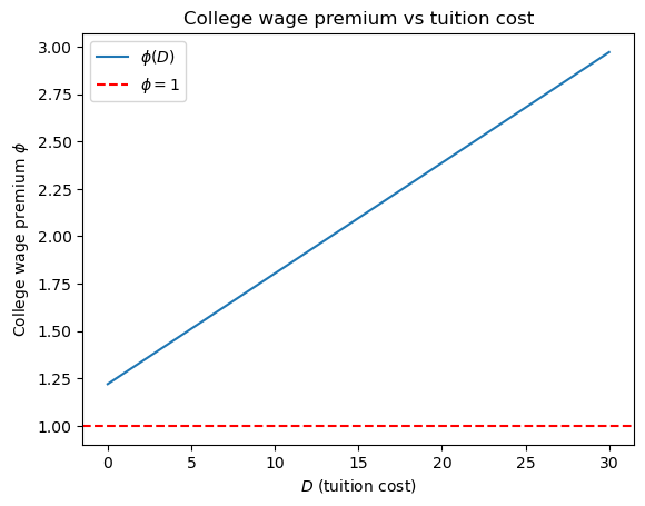
Using compute_gap, plot the college-high-school wage premium \(\phi\) as a function
of tuition cost \(D \in [0, 30]\) with all other parameters at their default values.
a. Add a horizontal dashed line at \(\phi = 1\) and explain why \(\phi\) does or does not reach 1 in this range in terms of the free-college formula \(\phi = A_h / A_c\).
b. Numerically estimate \(\partial\phi/\partial D\) as the slope of the plotted line and compare it to the symbolic derivative \(\phi_D\) computed with SymPy in this lecture.
Solution to Exercise 14.1
D_arr = np.linspace(0, 30, 200)
# Use create_edm_π with π=1 (certainty) so compute_gap handles the 7-field model
models = [create_edm_π(D=d, π=1.0) for d in D_arr]
gaps = [compute_gap(m) for m in models]

fig, ax = plt.subplots()
ax.plot(D_arr, gaps, label=r'$\phi(D)$')
ax.axhline(1, linestyle='--', color='red', label=r'$\phi = 1$')
ax.set_xlabel('$D$ (tuition cost)')
ax.set_ylabel(r'College wage premium $\phi$')
ax.set_title('College wage premium vs tuition cost')
ax.legend()
plt.show()

# Numerical slope (finite difference)
slope_num = (gaps[-1] - gaps[0]) / (D_arr[-1] - D_arr[0])

# Compare with SymPy ϕ_D_func already computed in this lecture
slope_sympy = float(ϕ_D_func(D_value, γ_h_value, γ_c_value, R_value, T_value, w_h0_value))

print(f'Numerical dϕ/dD: {slope_num:.6f}')
print(f'SymPy     dϕ/dD: {slope_sympy:.6f}')
print(f'Match: {abs(slope_num - slope_sympy) < 1e-4}')
Numerical dϕ/dD: 0.058368
SymPy     dϕ/dD: 0.058368
Match: True
Because \(A_h > A_c\) (forgone earnings dominate even with \(D=0\)), the free-college premium \(A_h/A_c > 1\), so \(\phi\) exceeds 1 for all \(D \geq 0\).
Exercise 14.2
Plot the college wage premium \(\phi\) as a function of career length \(T \in \{10, 15, 20, \ldots, 60\}\) for two cases:
Free college: \(D = 0\).
Costly college: \(D = 10\).
On the same graph, plot both curves, add a horizontal dashed line at \(\phi = 1\), and explain the direction of the relationship between \(T\) and \(\phi\) in terms of the present-value factors \(A_h\) and \(A_c\).
Solution to Exercise 14.2
T_arr = np.arange(10, 65, 5)

gaps_free   = [compute_gap(create_edm_π(T=t, D=0,  π=1.0)) for t in T_arr]
gaps_costly = [compute_gap(create_edm_π(T=t, D=10, π=1.0)) for t in T_arr]

fig, ax = plt.subplots()
ax.plot(T_arr, gaps_free,   'o-', label='$D = 0$ (free college)')
ax.plot(T_arr, gaps_costly, 's-', label='$D = 10$ (costly college)')
ax.axhline(1, linestyle='--', color='gray', label=r'$\phi = 1$')
ax.set_xlabel('Career length $T$')
ax.set_ylabel(r'College wage premium $\phi$')
ax.set_title('College wage premium vs career length')
ax.legend()
plt.show()
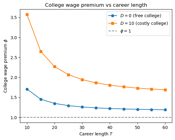
As \(T\) rises, college graduates have more years over which to “recoup” the cost of their four-year delay in starting work because \(A_c\) grows faster than \(A_h\) when the 4-year discount factor \((R^{-1}\gamma_c)^4\) is amortised over more periods.
This shrinks \(A_h/A_c\) and therefore \(\phi\).
Exercise 14.3
Verify the SymPy partial derivative \(\partial\phi/\partial R\) numerically using a central finite-difference approximation
for \(\varepsilon = 10^{-5}\), evaluating at the default parameter values and comparing with the symbolic result computed in this lecture.
Solution to Exercise 14.3
ε = 1e-5

# Finite-difference estimate using create_edm_π (π=1 for the standard model)
gap_plus  = compute_gap(create_edm_π(R=R_value + ε, π=1.0))
gap_minus = compute_gap(create_edm_π(R=R_value - ε, π=1.0))
dϕ_dR_fd  = (gap_plus - gap_minus) / (2 * ε)

# SymPy result from ϕ_R_func already computed in this lecture
dϕ_dR_sym = float(ϕ_R_func(D_value, γ_h_value, γ_c_value, R_value, T_value, w_h0_value))

print(f'Finite-difference dϕ/dR: {dϕ_dR_fd:.6f}')
print(f'SymPy             dϕ/dR: {dϕ_dR_sym:.6f}')
print(f'Absolute error:           {abs(dϕ_dR_fd - dϕ_dR_sym):.2e}')
Finite-difference dϕ/dR: 13.264274
SymPy             dϕ/dR: 13.264274
Absolute error:           1.89e-09
The two estimates agree to at least five significant figures, confirming that the symbolic calculus and numerical computation are consistent.
Exercise 14.4
Using the entrepreneur-worker version of the model (create_edm_π), answer the
following questions.
a. Plot the required wage premium \(\phi\) for a successful entrepreneur as a function of the success probability \(\pi \in [0.10, 1.00]\) and mark the horizontal line \(\phi = 2\) as a dashed line.
b. At what approximate value of \(\pi\) does the premium cross 2, and for which side of that threshold is the premium above 2?
c. Explain intuitively why the premium rises as \(\pi \to 0\).
Solution to Exercise 14.4
π_arr = np.linspace(0.10, 1.00, 200)
# create_edm_π and compute_gap are already defined in this lecture
ϕ_arr_π = np.array([compute_gap(create_edm_π(π=p)) for p in π_arr])

fig, ax = plt.subplots()
ax.plot(π_arr, ϕ_arr_π, label=r'$\phi(\pi)$')
ax.axhline(2, linestyle='--', color='red', label=r'$\phi = 2$')
ax.set_xlabel(r'Success probability $\pi$')
ax.set_ylabel(r'Required wage premium $\phi$')
ax.set_title('Entrepreneur premium vs success probability')
ax.legend()
plt.show()

# Interpolate the crossing on the decreasing curve ϕ(π)
crossing = np.interp(2, ϕ_arr_π[::-1], π_arr[::-1])
above_idx = np.where(ϕ_arr_π > 2)[0]

print(f'Premium equals 2 at π approximately {crossing:.3f}')
print(f'On the grid, premium exceeds 2 for π below about {π_arr[above_idx[-1]]:.3f}')
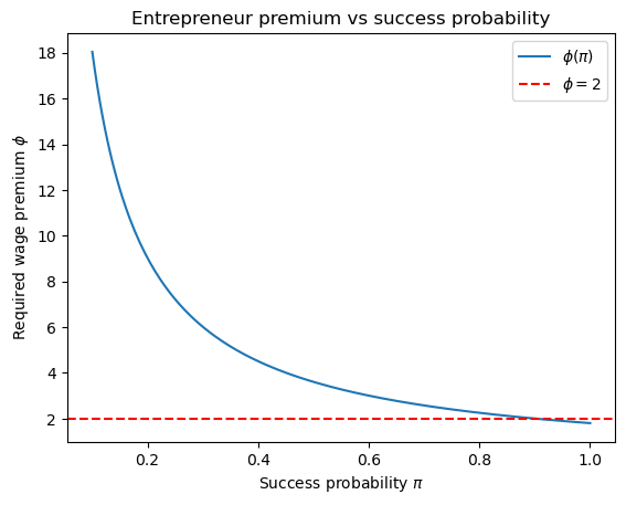
Premium equals 2 at π approximately 0.902
On the grid, premium exceeds 2 for π below about 0.901
As \(\pi \to 0\) the expected lifetime earnings of an entrepreneur approach zero regardless of \(\phi\), so \(\phi\) must rise without bound to keep the entrepreneur indifferent between entrepreneurship and wage work.