10. Geometric Series for Elementary Economics#
10.1. Overview#
The lecture describes important ideas in economics that use the mathematics of geometric series.
Among these are
the Keynesian multiplier
the money multiplier that prevails in fractional reserve banking systems
interest rates and present values of streams of payouts from assets
(As we shall see below, the term multiplier comes down to meaning sum of a convergent geometric series)
These and other applications prove the truth of the wise crack that
“In economics, a little knowledge of geometric series goes a long way.”
Below we’ll use the following imports:
import matplotlib.pyplot as plt
plt.rcParams["figure.figsize"] = (11, 5)  #set default figure size
import numpy as np
import sympy as sym
from sympy import init_printing
from matplotlib import cm
10.2. Key formulas#
To start, let \(c\) be a real number that lies strictly between \(-1\) and \(1\).
We often write this as \(c \in (-1,1)\).
Here \((-1,1)\) denotes the collection of all real numbers that are strictly less than \(1\) and strictly greater than \(-1\).
The symbol \(\in\) means in or belongs to the set after the symbol.
We want to evaluate geometric series of two types – infinite and finite.
10.2.1. Infinite geometric series#
The first type of geometric that interests us is the infinite series
Where \(\cdots\) means that the series continues without end.
The key formula is
To prove key formula (10.1), multiply both sides by \((1-c)\) and verify that if \(c \in (-1,1)\), then the outcome is the equation \(1 = 1\).
10.2.2. Finite geometric series#
The second series that interests us is the finite geometric series
where \(T\) is a positive integer.
The key formula here is
Remark 10.1
The above formula works for any value of the scalar \(c\). We don’t have to restrict \(c\) to be in the set \((-1,1)\).
We now move on to describe some famous economic applications of geometric series.
10.3. Example: The Money Multiplier in Fractional Reserve Banking#
In a fractional reserve banking system, banks hold only a fraction \(r \in (0,1)\) of cash behind each deposit receipt that they issue
In recent times
cash consists of pieces of paper issued by the government and called dollars or pounds or \(\ldots\)
a deposit is a balance in a checking or savings account that entitles the owner to ask the bank for immediate payment in cash
When the UK and France and the US were on either a gold or silver standard (before 1914, for example)
cash was a gold or silver coin
a deposit receipt was a bank note that the bank promised to convert into gold or silver on demand; (sometimes it was also a checking or savings account balance)
Economists and financiers often define the supply of money as an economy-wide sum of cash plus deposits.
In a fractional reserve banking system (one in which the reserve ratio \(r\) satisfies \(0 < r < 1\)), banks create money by issuing deposits backed by fractional reserves plus loans that they make to their customers.
A geometric series is a key tool for understanding how banks create money (i.e., deposits) in a fractional reserve system.
The geometric series formula (10.1) is at the heart of the classic model of the money creation process – one that leads us to the celebrated money multiplier.
10.3.1. A simple model#
There is a set of banks named \(i = 0, 1, 2, \ldots\).
Bank \(i\)’s loans \(L_i\), deposits \(D_i\), and reserves \(R_i\) must satisfy the balance sheet equation (because balance sheets balance):
The left side of the above equation is the sum of the bank’s assets, namely, the loans \(L_i\) it has outstanding plus its reserves of cash \(R_i\).
The right side records bank \(i\)’s liabilities, namely, the deposits \(D_i\) held by its depositors; these are IOU’s from the bank to its depositors in the form of either checking accounts or savings accounts (or before 1914, bank notes issued by a bank stating promises to redeem notes for gold or silver on demand).
Each bank \(i\) sets its reserves to satisfy the equation
where \(r \in (0,1)\) is its reserve-deposit ratio or reserve ratio for short
the reserve ratio is either set by a government or chosen by banks for precautionary reasons
Next we add a theory stating that bank \(i+1\)’s deposits depend entirely on loans made by bank \(i\), namely
Thus, we can think of the banks as being arranged along a line with loans from bank \(i\) being immediately deposited in \(i+1\)
in this way, the debtors to bank \(i\) become creditors of bank \(i+1\)
Finally, we add an initial condition about an exogenous level of bank \(0\)’s deposits
We can think of \(D_0\) as being the amount of cash that a first depositor put into the first bank in the system, bank number \(i=0\).
Now we do a little algebra.
Combining equations (10.2) and (10.3) tells us that
This states that bank \(i\) loans a fraction \((1-r)\) of its deposits and keeps a fraction \(r\) as cash reserves.
Combining equation (10.5) with equation (10.4) tells us that
which implies that
Equation (10.6) expresses \(D_i\) as the \(i\) th term in the product of \(D_0\) and the geometric series
Therefore, the sum of all deposits in our banking system \(i=0, 1, 2, \ldots\) is
10.3.2. Money multiplier#
The money multiplier is a number that tells the multiplicative factor by which an exogenous injection of cash into bank \(0\) leads to an increase in the total deposits in the banking system.
Equation (10.7) asserts that the money multiplier is \(\frac{1}{r}\)
An initial deposit of cash of \(D_0\) in bank \(0\) leads the banking system to create total deposits of \(\frac{D_0}{r}\).
The initial deposit \(D_0\) is held as reserves, distributed throughout the banking system according to \(D_0 = \sum_{i=0}^\infty R_i\).
10.4. Example: The Keynesian Multiplier#
The famous economist John Maynard Keynes and his followers created a simple model intended to determine national income \(y\) in circumstances in which
there are substantial unemployed resources, in particular excess supply of labor and capital
prices and interest rates fail to adjust to make aggregate supply equal demand (e.g., prices and interest rates are frozen)
national income is entirely determined by aggregate demand
10.4.1. Static version#
An elementary Keynesian model of national income determination consists of three equations that describe aggregate demand for \(y\) and its components.
The first equation is a national income identity asserting that consumption \(c\) plus investment \(i\) equals national income \(y\):
The second equation is a Keynesian consumption function asserting that people consume a fraction \(b \in (0,1)\) of their income:
The fraction \(b \in (0,1)\) is called the marginal propensity to consume.
The fraction \(1-b \in (0,1)\) is called the marginal propensity to save.
The third equation simply states that investment is exogenous at level \(i\).
exogenous means determined outside this model.
Substituting the second equation into the first gives \((1-b) y = i\).
Solving this equation for \(y\) gives
The quantity \(\frac{1}{1-b}\) is called the investment multiplier or simply the multiplier.
Applying the formula for the sum of an infinite geometric series, we can write the above equation as
where \(t\) is a nonnegative integer.
So we arrive at the following equivalent expressions for the multiplier:
The expression \(\sum_{t=0}^\infty b^t\) motivates an interpretation of the multiplier as the outcome of a dynamic process that we describe next.
10.4.2. Dynamic version#
We arrive at a dynamic version by interpreting the nonnegative integer \(t\) as indexing time and changing our specification of the consumption function to take time into account
we add a one-period lag in how income affects consumption
We let \(c_t\) be consumption at time \(t\) and \(i_t\) be investment at time \(t\).
We modify our consumption function to assume the form
so that \(b\) is the marginal propensity to consume (now) out of last period’s income.
We begin with an initial condition stating that
We also assume that
so that investment is constant over time.
It follows that
and
and
and more generally
or
Evidently, as \(t \rightarrow + \infty\),
Remark 1: The above formula is often applied to assert that an exogenous increase in investment of \(\Delta i\) at time \(0\) ignites a dynamic process of increases in national income by successive amounts
at times \(0, 1, 2, \ldots\).
Remark 2 Let \(g_t\) be an exogenous sequence of government expenditures.
If we generalize the model so that the national income identity becomes
then a version of the preceding argument shows that the government expenditures multiplier is also \(\frac{1}{1-b}\), so that a permanent increase in government expenditures ultimately leads to an increase in national income equal to the multiplier times the increase in government expenditures.
10.5. Example: Interest Rates and Present Values#
We can apply our formula for geometric series to study how interest rates affect values of streams of dollar payments that extend over time.
We work in discrete time and assume that \(t = 0, 1, 2, \ldots\) indexes time.
We let \(r \in (0,1)\) be a one-period net nominal interest rate
if the nominal interest rate is \(5\) percent, then \(r= .05\)
A one-period gross nominal interest rate \(R\) is defined as
if \(r=.05\), then \(R = 1.05\)
Remark: The gross nominal interest rate \(R\) is an exchange rate or relative price of dollars between times \(t\) and \(t+1\). The units of \(R\) are dollars at time \(t+1\) per dollar at time \(t\).
When people borrow and lend, they trade dollars now for dollars later or dollars later for dollars now.
The price at which these exchanges occur is the gross nominal interest rate.
If I sell \(x\) dollars to you today, you pay me \(R x\) dollars tomorrow.
This means that you borrowed \(x\) dollars from me at a gross interest rate \(R\) and a net interest rate \(r\).
We assume that the net nominal interest rate \(r\) is fixed over time, so that \(R\) is the gross nominal interest rate at times \(t=0, 1, 2, \ldots\).
Two important geometric sequences are
and
Sequence (10.8) tells us how dollar values of an investment accumulate through time.
Sequence (10.9) tells us how to discount future dollars to get their values in terms of today’s dollars.
10.5.1. Accumulation#
Geometric sequence (10.8) tells us how one dollar invested and re-invested in a project with gross one period nominal rate of return accumulates
here we assume that net interest payments are reinvested in the project
thus, \(1\) dollar invested at time \(0\) pays interest \(r\) dollars after one period, so we have \(r+1 = R\) dollars at time\(1\)
at time \(1\) we reinvest \(1+r =R\) dollars and receive interest of \(r R\) dollars at time \(2\) plus the principal \(R\) dollars, so we receive \(r R + R = (1+r)R = R^2\) dollars at the end of period \(2\)
and so on
Evidently, if we invest \(x\) dollars at time \(0\) and reinvest the proceeds, then the sequence
tells how our account accumulates at dates \(t=0, 1, 2, \ldots\).
10.5.2. Discounting#
Geometric sequence (10.9) tells us how much future dollars are worth in terms of today’s dollars.
Remember that the units of \(R\) are dollars at \(t+1\) per dollar at \(t\).
It follows that
the units of \(R^{-1}\) are dollars at \(t\) per dollar at \(t+1\)
the units of \(R^{-2}\) are dollars at \(t\) per dollar at \(t+2\)
and so on; the units of \(R^{-j}\) are dollars at \(t\) per dollar at \(t+j\)
So if someone has a claim on \(x\) dollars at time \(t+j\), it is worth \(x R^{-j}\) dollars at time \(t\) (e.g., today).
10.5.3. Application to asset pricing#
A lease requires a payments stream of \(x_t\) dollars at times \(t = 0, 1, 2, \ldots\) where
where \(G = (1+g)\) and \(g \in (0,1)\).
Thus, lease payments increase at \(g\) percent per period.
For a reason soon to be revealed, we assume that \(G < R\).
The present value of the lease is
where the last line uses the formula for an infinite geometric series.
Recall that \(R = 1+r\) and \(G = 1+g\) and that \(R > G\) and \(r > g\) and that \(r\) and \(g\) are typically small numbers, e.g., .05 or .03.
Use the Taylor series of \(\frac{1}{1+r}\) about \(r=0\), namely,
and the fact that \(r\) is small to approximate \(\frac{1}{1+r} \approx 1 - r\).
Use this approximation to write \(p_0\) as
where the last step uses the approximation \(r g \approx 0\).
The approximation
is known as the Gordon formula for the present value or current price of an infinite payment stream \(x_0 G^t\) when the nominal one-period interest rate is \(r\) and when \(r > g\).
We can also extend the asset pricing formula so that it applies to finite leases.
Let the payment stream on the lease now be \(x_t\) for \(t= 1,2, \dots,T\), where again
The present value of this lease is:
Applying the Taylor series to \(R^{-(T+1)}\) about \(r=0\) we get:
Similarly, applying the Taylor series to \(G^{T+1}\) about \(g=0\):
Thus, we get the following approximation:
Expanding:
We could have also approximated by removing the second term \(rgx_0(T+1)\) when \(T\) is relatively small compared to \(1/(rg)\) to get \(x_0(T+1)\) as in the finite stream approximation.
We will plot the true finite stream present-value and the two approximations, under different values of \(T\), and \(g\) and \(r\) in Python.
First we plot the true finite stream present-value after computing it below
# True present value of a finite lease
def finite_lease_pv_true(T, g, r, x_0):
    G = (1 + g)
    R = (1 + r)
    return (x_0 * (1 - G**(T + 1) * R**(-T - 1))) / (1 - G * R**(-1))
# First approximation for our finite lease

def finite_lease_pv_approx_1(T, g, r, x_0):
    p = x_0 * (T + 1) + x_0 * r * g * (T + 1) / (r - g)
    return p

# Second approximation for our finite lease
def finite_lease_pv_approx_2(T, g, r, x_0):
    return (x_0 * (T + 1))

# Infinite lease
def infinite_lease(g, r, x_0):
    G = (1 + g)
    R = (1 + r)
    return x_0 / (1 - G * R**(-1))
Now that we have defined our functions, we can plot some outcomes.
First we study the quality of our approximations
def plot_function(axes, x_vals, func, args):
    axes.plot(x_vals, func(*args), label=func.__name__)

T_max = 50

T = np.arange(0, T_max+1)
g = 0.02
r = 0.03
x_0 = 1

our_args = (T, g, r, x_0)
funcs = [finite_lease_pv_true,
        finite_lease_pv_approx_1,
        finite_lease_pv_approx_2]
        # the three functions we want to compare

fig, ax = plt.subplots()
for f in funcs:
    plot_function(ax, T, f, our_args)
ax.legend()
ax.set_xlabel('$T$ Periods Ahead')
ax.set_ylabel('Present Value, $p_0$')
plt.show()
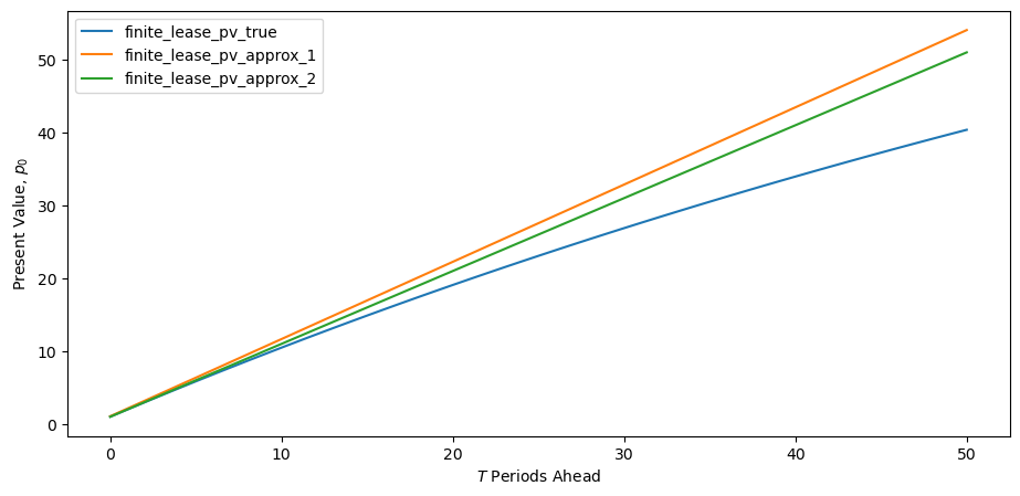
Fig. 10.1 Finite lease present value \(T\) periods ahead#
Evidently our approximations perform well for small values of \(T\).
However, holding \(g\) and r fixed, our approximations deteriorate as \(T\) increases.
Next we compare the infinite and finite duration lease present values over different lease lengths \(T\).
# Convergence of infinite and finite
T_max = 1000
T = np.arange(0, T_max+1)
fig, ax = plt.subplots()
f_1 = finite_lease_pv_true(T, g, r, x_0)
f_2 = np.full(T_max+1, infinite_lease(g, r, x_0))
ax.plot(T, f_1, label='T-period lease PV')
ax.plot(T, f_2, '--', label='Infinite lease PV')
ax.set_xlabel('$T$ Periods Ahead')
ax.set_ylabel('Present Value, $p_0$')
ax.legend()
plt.show()
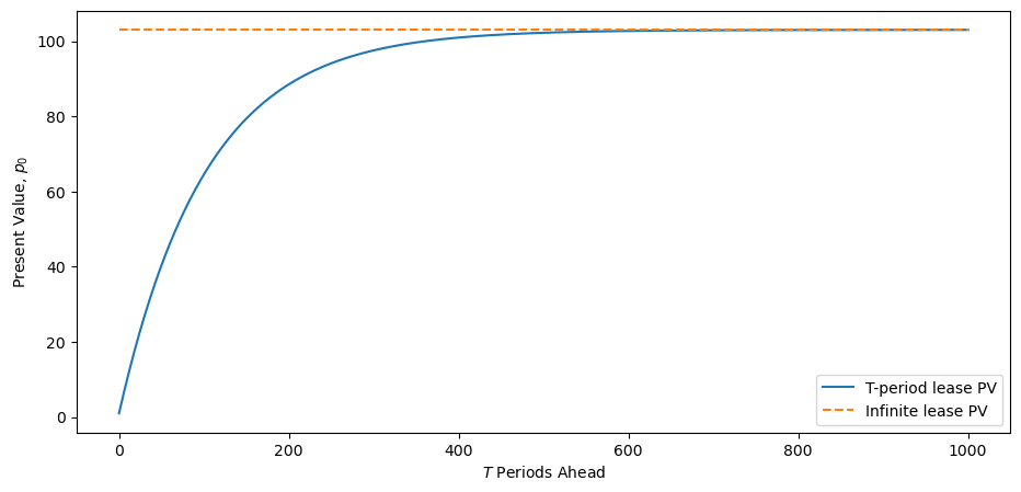
Fig. 10.2 Infinite and finite lease present value \(T\) periods ahead#
The graph above shows how as duration \(T \rightarrow +\infty\), the value of a lease of duration \(T\) approaches the value of a perpetual lease.
Now we consider two different views of what happens as \(r\) and \(g\) covary
# First view
# Changing r and g
fig, ax = plt.subplots()
ax.set_ylabel('Present Value, $p_0$')
ax.set_xlabel('$T$ periods ahead')
T_max = 10
T=np.arange(0, T_max+1)

rs, gs = (0.9, 0.5, 0.4001, 0.4), (0.4, 0.4, 0.4, 0.5),
comparisons = (r'$\gg$', '$>$', r'$\approx$', '$<$')
for r, g, comp in zip(rs, gs, comparisons):
    ax.plot(finite_lease_pv_true(T, g, r, x_0), label=f'r(={r}) {comp} g(={g})')

ax.legend()
plt.show()
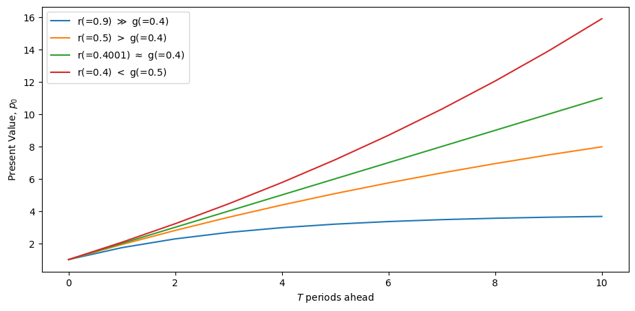
Fig. 10.3 Value of lease of length \(T\)#
This graph gives a big hint for why the condition \(r > g\) is necessary if a lease of length \(T = +\infty\) is to have finite value.
For fans of 3-d graphs the same point comes through in the following graph.
If you aren’t enamored of 3-d graphs, feel free to skip the next visualization!
# Second view
fig = plt.figure(figsize = [16, 5])
T = 3
ax = plt.subplot(projection='3d')
r = np.arange(0.01, 0.99, 0.005)
g = np.arange(0.011, 0.991, 0.005)

rr, gg = np.meshgrid(r, g)
z = finite_lease_pv_true(T, gg, rr, x_0)

# Removes points where undefined
same = (rr == gg)
z[same] = np.nan
surf = ax.plot_surface(rr, gg, z, cmap=cm.coolwarm,
    antialiased=True, clim=(0, 15))
fig.colorbar(surf, shrink=0.5, aspect=5)
ax.set_xlabel('$r$')
ax.set_ylabel('$g$')
ax.set_zlabel('Present Value, $p_0$')
ax.view_init(20, 8)
plt.show()
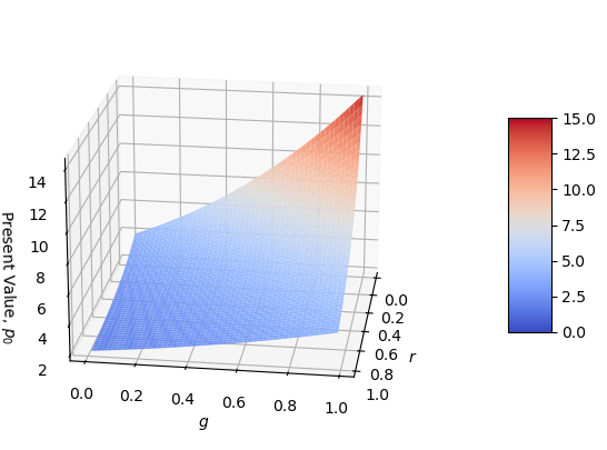
Fig. 10.4 Three period lease PV with varying \(g\) and \(r\)#
We can use a little calculus to study how the present value \(p_0\) of a lease varies with \(r\) and \(g\).
We will use a library called SymPy.
SymPy enables us to do symbolic math calculations including computing derivatives of algebraic equations.
We will illustrate how it works by creating a symbolic expression that represents our present value formula for an infinite lease.
After that, we’ll use SymPy to compute derivatives
# Creates algebraic symbols that can be used in an algebraic expression
g, r, x0 = sym.symbols('g, r, x0')
G = (1 + g)
R = (1 + r)
p0 = x0 / (1 - G * R**(-1))
init_printing(use_latex='mathjax')
print('Our formula is:')
p0
Our formula is:
print('dp0 / dg is:')
dp_dg = sym.diff(p0, g)
dp_dg
dp0 / dg is:
print('dp0 / dr is:')
dp_dr = sym.diff(p0, r)
dp_dr
dp0 / dr is:
We can see that for \(\frac{\partial p_0}{\partial r}<0\) as long as \(r>g\), \(r>0\) and \(g>0\) and \(x_0\) is positive, so \(\frac{\partial p_0}{\partial r}\) will always be negative.
Similarly, \(\frac{\partial p_0}{\partial g}>0\) as long as \(r>g\), \(r>0\) and \(g>0\) and \(x_0\) is positive, so \(\frac{\partial p_0}{\partial g}\) will always be positive.
10.6. Back to the Keynesian multiplier#
We will now go back to the case of the Keynesian multiplier and plot the time path of \(y_t\), given that consumption is a constant fraction of national income, and investment is fixed.
# Function that calculates a path of y
def calculate_y(i, b, g, T, y_init):
    y = np.zeros(T+1)
    y[0] = i + b * y_init + g
    for t in range(1, T+1):
        y[t] = b * y[t-1] + i + g
    return y

# Initial values
i_0 = 0.3
g_0 = 0.3
# 2/3 of income goes towards consumption
b = 2/3
y_init = 0
T = 100

fig, ax = plt.subplots()
ax.set_xlabel('$t$')
ax.set_ylabel('$y_t$')
ax.plot(np.arange(0, T+1), calculate_y(i_0, b, g_0, T, y_init))
# Output predicted by geometric series
ax.hlines(i_0 / (1 - b) + g_0 / (1 - b), xmin=-1, xmax=101, linestyles='--')
plt.show()
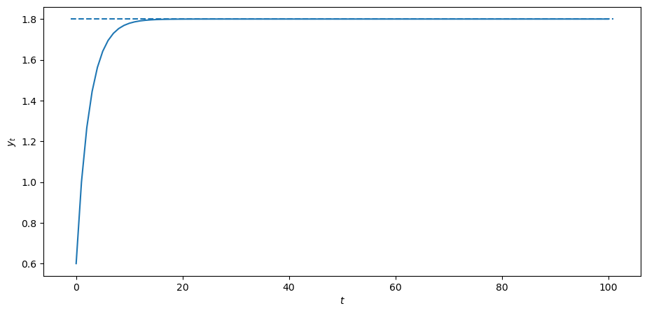
Fig. 10.5 Path of aggregate output over time#
In this model, income grows over time, until it gradually converges to the infinite geometric series sum of income.
We now examine what will happen if we vary the so-called marginal propensity to consume, i.e., the fraction of income that is consumed
bs = (1/3, 2/3, 5/6, 0.9)

fig,ax = plt.subplots()
ax.set_ylabel('$y_t$')
ax.set_xlabel('$t$')
x = np.arange(0, T+1)
for b in bs:
    y = calculate_y(i_0, b, g_0, T, y_init)
    ax.plot(x, y, label=r'$b=$'+f"{b:.2f}")
ax.legend()
plt.show()
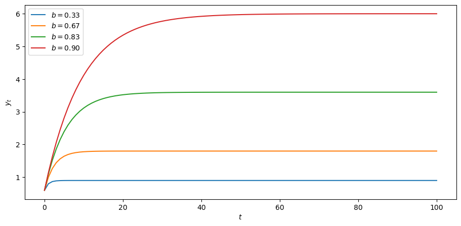
Fig. 10.6 Changing consumption as a fraction of income#
Increasing the marginal propensity to consume \(b\) increases the path of output over time.
Now we will compare the effects on output of increases in investment and government spending.
fig, (ax1, ax2) = plt.subplots(2, 1, figsize=(6, 10))
fig.subplots_adjust(hspace=0.3)

x = np.arange(0, T+1)
values = [0.3, 0.4]

for i in values:
    y = calculate_y(i, b, g_0, T, y_init)
    ax1.plot(x, y, label=f"i={i}")
for g in values:
    y = calculate_y(i_0, b, g, T, y_init)
    ax2.plot(x, y, label=f"g={g}")

axes = ax1, ax2
param_labels = "Investment", "Government Spending"
for ax, param in zip(axes, param_labels):
    ax.set_title(f'An Increase in {param} on Output')
    ax.legend(loc ="lower right")
    ax.set_ylabel('$y_t$')
    ax.set_xlabel('$t$')
plt.show()
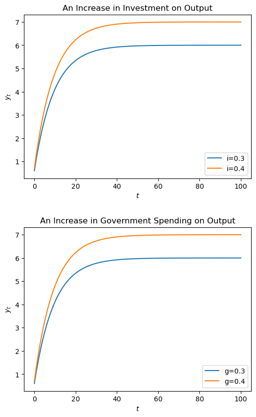
Fig. 10.7 Different increase on output#
Notice here, whether government spending increases from 0.3 to 0.4 or investment increases from 0.3 to 0.4, the shifts in the graphs are identical.
10.7. Exercises#
Exercise 10.1
Numerically verify the infinite geometric series formula
for \(c = 0.9\).
Compute the partial sums \(S_T = \sum_{t=0}^{T} c^t\) for \(T = 0, 1, \ldots, 80\) and plot them alongside the theoretical limit \(\frac{1}{1-c}\).
On a second subplot, plot the absolute error \(\left|S_T - \frac{1}{1-c}\right|\) on a log scale to illustrate the rate of convergence.
Solution
c = 0.9
T_max = 80
T = np.arange(0, T_max + 1)

# Partial sums: S_T = sum_{t=0}^{T} c^t
S = np.cumsum(c**T)

# Theoretical limit
limit = 1 / (1 - c)

fig, axes = plt.subplots(1, 2, figsize=(12, 4))

# Left panel: partial sums converging to the limit
axes[0].plot(T, S, label='Partial sum $S_T$')
axes[0].axhline(limit, linestyle='--', color='red',
                label=f'Limit $1/(1-c) = {limit:.1f}$')
axes[0].set_xlabel('$T$')
axes[0].set_ylabel('$S_T$')
axes[0].set_title('Convergence of partial sums')
axes[0].legend()

# Right panel: absolute error on log scale
error = np.abs(S - limit)
axes[1].semilogy(T, error)
axes[1].set_xlabel('$T$')
axes[1].set_ylabel(r'$|S_T - 1/(1-c)|$')
axes[1].set_title('Absolute error (log scale)')

plt.tight_layout()
plt.show()
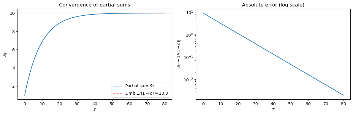
The left panel confirms that \(S_T\) converges smoothly to \(1/(1-c) = 10\).
The right panel shows that the error decays geometrically, a straight line on a log scale, reflecting the fact that the remainder after \(T\) terms equals \(c^{T+1}/(1-c)\).
Exercise 10.2
Using the fractional reserve banking model from this lecture, suppose the initial deposit is \(D_0 = 1\).
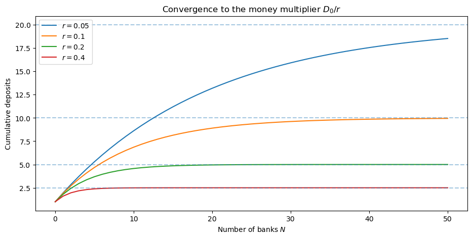
a. For each reserve ratio \(r \in \{0.05, 0.10, 0.20, 0.40\}\), plot the cumulative deposits \(\sum_{i=0}^{N} D_i\) as a function of the number of banks \(N\) (for \(N = 0, 1, \ldots, 50\)) and add a dashed horizontal line at the theoretical limit \(D_0/r\) for each.
b. Print the theoretical money multiplier \(1/r\) for each reserve ratio.
Solution
D_0 = 1
N_max = 50
N = np.arange(0, N_max + 1)
reserve_ratios = [0.05, 0.10, 0.20, 0.40]

fig, ax = plt.subplots()
for r in reserve_ratios:
    # D_i = (1 - r)^i * D_0
    D = D_0 * (1 - r)**N
    cumulative = np.cumsum(D)
    ax.plot(N, cumulative, label=f'$r = {r}$')
    ax.axhline(D_0 / r, linestyle='--', alpha=0.4)

ax.set_xlabel('Number of banks $N$')
ax.set_ylabel('Cumulative deposits')
ax.set_title('Convergence to the money multiplier $D_0/r$')
ax.legend()
plt.show()

# Part b
print(f"{'Reserve ratio':>15} | {'Money multiplier 1/r':>20}")
print('-' * 40)
for r in reserve_ratios:
    print(f"{r:>15.2f} | {1/r:>20.2f}")
  Reserve ratio | Money multiplier 1/r
----------------------------------------
           0.05 |                20.00
           0.10 |                10.00
           0.20 |                 5.00
           0.40 |                 2.50
A lower reserve ratio means banks lend out a larger fraction of each deposit, so the money-creation process takes longer to run down and the total deposits created are much larger.
The dashed lines mark the theoretical limit \(D_0/r\), which the cumulative series approaches from below.
Exercise 10.3
The Gordon formula approximates the present value of an infinite lease as
Using the infinite_lease function defined earlier, set \(x_0 = 1\) and
\(r = 0.05\), and let \(g\) range over \([0,\, 0.045]\).
a. Plot the exact present value and the Gordon approximation on the same graph as functions of \(g\).
b. On a second subplot, plot the percentage approximation error
and comment on whether the percentage error varies with \(g\).
Solution
r_val = 0.05
x_0 = 1
g_vals = np.linspace(0, 0.045, 300)

exact = infinite_lease(g_vals, r_val, x_0)
gordon = x_0 / (r_val - g_vals)
pct_error = np.abs(gordon - exact) / exact * 100
pct_error_formula = 100 * r_val / (1 + r_val)

fig, axes = plt.subplots(1, 2, figsize=(12, 4))

axes[0].plot(g_vals, exact, label='Exact $p_0$')
axes[0].plot(g_vals, gordon, '--', label='Gordon approximation')
axes[0].set_xlabel('$g$')
axes[0].set_ylabel('$p_0$')
axes[0].set_title(f'Infinite lease present value ($r = {r_val}$)')
axes[0].legend()

axes[1].plot(g_vals, pct_error)
axes[1].axhline(pct_error_formula, linestyle='--', color='red',
                label=fr'$100r/(1+r) = {pct_error_formula:.2f}\%$')
axes[1].set_xlabel('$g$')
axes[1].set_ylabel('Percentage error (%)')
axes[1].set_title('Gordon formula approximation error')
axes[1].legend()

plt.tight_layout()
plt.show()
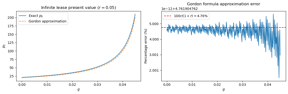
For a fixed \(r\), the percentage error is constant in \(g\) because the exact value is \(x_0(1+r)/(r-g)\) while the Gordon approximation is \(x_0/(r-g)\).
The approximation becomes accurate when \(r\) is small because the exact value differs from the Gordon formula by the factor \(1+r\).
Exercise 10.4
The calculate_y function simulates the Keynesian dynamic model.
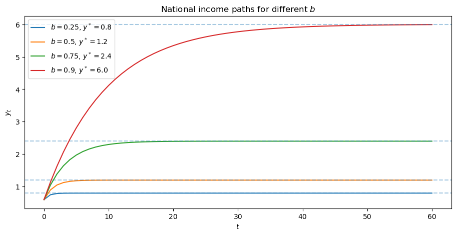
a. For \(i = 0.3\), \(g = 0.3\), \(y_{-1} = 0\), and \(T = 60\), plot the path of national income \(y_t\) for each \(b \in \{0.25,\, 0.50,\, 0.75,\, 0.90\}\) and mark the long-run equilibrium \(y^* = (i + g)/(1 - b)\) with a dashed horizontal line for each \(b\).
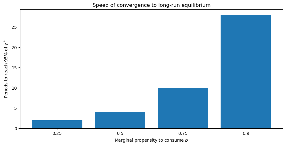
b. For each value of \(b\), find the first period \(T^*\) at which \(y_t\) reaches 95 percent of \(y^*\), plot \(T^*\) against \(b\), and comment on how the speed of convergence relates to the size of the Keynesian multiplier.
Solution
i_0, g_0, y_init = 0.3, 0.3, 0
bs = [0.25, 0.50, 0.75, 0.90]
T = 60

# Part a
fig, ax = plt.subplots()
for b in bs:
    y = calculate_y(i_0, b, g_0, T, y_init)
    y_star = (i_0 + g_0) / (1 - b)
    ax.plot(np.arange(T + 1), y, label=f'$b = {b}$, $y^* = {y_star:.1f}$')
    ax.axhline(y_star, linestyle='--', alpha=0.4)

ax.set_xlabel('$t$')
ax.set_ylabel('$y_t$')
ax.set_title('National income paths for different $b$')
ax.legend()
plt.show()

# Part b
T_long = 1000
T_star_vals = []
for b in bs:
    y = calculate_y(i_0, b, g_0, T_long, y_init)
    y_star = (i_0 + g_0) / (1 - b)
    idx = np.where(y >= 0.95 * y_star)[0]
    T_star_vals.append(int(idx[0]) if len(idx) > 0 else T_long)

fig, ax = plt.subplots()
ax.bar([str(b) for b in bs], T_star_vals)
ax.set_xlabel('Marginal propensity to consume $b$')
ax.set_ylabel('Periods to reach 95% of $y^*$')
ax.set_title('Speed of convergence to long-run equilibrium')
plt.show()

print(f"{'b':>6} | {'Multiplier 1/(1-b)':>20} | {'T* (periods)':>14}")
print('-' * 46)
for b, T_star in zip(bs, T_star_vals):
    print(f"{b:>6.2f} | {1/(1-b):>20.2f} | {T_star:>14}")
     b |   Multiplier 1/(1-b) |   T* (periods)
----------------------------------------------
  0.25 |                 1.33 |              2
  0.50 |                 2.00 |              4
  0.75 |                 4.00 |             10
  0.90 |                10.00 |             28
As \(b\) rises toward 1, the Keynesian multiplier \(1/(1-b)\) grows large and convergence slows markedly.
This reflects the fact that the geometric series \(\sum_{t=0}^\infty b^t\) converges more slowly when \(b\) is close to 1 because each additional round of spending adds a term \(b^t\) that shrinks only gradually.