31. Some Unpleasant Monetarist Arithmetic#
31.1. Overview#
This lecture builds on concepts and issues introduced in Money Financed Government Deficits and Price Levels.
That lecture describes stationary equilibria that reveal a Laffer curve in the inflation tax rate and the associated stationary rate of return on currency.
In this lecture we study a situation in which a stationary equilibrium prevails after date \(T > 0\), but not before then.
For \(t=0, \ldots, T-1\), the money supply, price level, and interest-bearing government debt vary along a transition path that ends at \(t=T\).
During this transition, the ratio of the real balances \(\frac{m_{t+1}}{{p_t}}\) to indexed one-period government bonds \(\tilde R B_{t-1}\) maturing at time \(t\) decreases each period.
This has consequences for the gross-of-interest government deficit that must be financed by printing money for times \(t \geq T\).
The critical money-to-bonds ratio stabilizes only at time \(T\) and afterwards.
And the larger is \(T\), the higher is the gross-of-interest government deficit that must be financed by printing money at times \(t \geq T\).
These outcomes are the essential finding of Sargent and Wallace’s “unpleasant monetarist arithmetic” [Sargent and Wallace, 1981].
That lecture described supplies and demands for money that appear in that lecture.
It also characterized the steady state equilibrium from which we work backwards in this lecture.
In addition to learning about “unpleasant monetarist arithmetic”, in this lecture we’ll learn how to implement a fixed point algorithm for computing an initial price level.
31.2. Setup#
Let’s start with quick reminders of the model’s components set out in Money Financed Government Deficits and Price Levels.
Please consult that lecture for more details and Python code that we’ll also use in this lecture.
For \(t \geq 1\), real balances evolve according to
or
where
\(b_t = \frac{m_{t+1}}{p_t}\) is real balances at the end of period \(t\)
\(R_{t-1} = \frac{p_{t-1}}{p_t}\) is the gross rate of return on real balances held from \(t-1\) to \(t\)
The demand for real balances is
where \(\gamma_1 > \gamma_2 > 0\).
31.3. Monetary-Fiscal Policy#
To the basic model of Money Financed Government Deficits and Price Levels, we add inflation-indexed one-period government bonds as an additional way for the government to finance government expenditures.
Let \(\widetilde R > 1\) be a time-invariant gross real rate of return on government one-period inflation-indexed bonds.
With this additional source of funds, the government’s budget constraint at time \(t \geq 0\) is now
Just before the beginning of time \(0\), the public owns \(\check m_0\) units of currency (measured in dollars) and \(\widetilde R \check B_{-1}\) units of one-period indexed bonds (measured in time \(0\) goods); these two quantities are initial conditions set outside the model.
Notice that \(\check m_0\) is a nominal quantity, being measured in dollars, while \(\widetilde R \check B_{-1}\) is a real quantity, being measured in time \(0\) goods.
31.3.1. Open market operations#
At time \(0\), government can rearrange its portfolio of debts subject to the following constraint (on open-market operations):
or
This equation says that the government (e.g., the central bank) can decrease \(m_0\) relative to \(\check m_0\) by increasing \(B_{-1}\) relative to \(\check B_{-1}\).
This is a version of a standard constraint on a central bank’s open market operations in which it expands the stock of money by buying government bonds from the public.
31.4. An open market operation at \(t=0\)#
Following Sargent and Wallace [Sargent and Wallace, 1981], we analyze consequences of a central bank policy that uses an open market operation to lower the price level in the face of a persistent fiscal deficit that takes the form of a positive \(g\).
Just before time \(0\), the government chooses \((m_0, B_{-1})\) subject to constraint (31.3).
For \(t =0, 1, \ldots, T-1\),
while for \(t \geq T\),
where
We want to compute an equilibrium \(\{p_t,m_t,b_t, R_t\}_{t=0}\) sequence under this scheme for running monetary and fiscal policies.
Here, by fiscal policy we mean the collection of actions that determine a sequence of net-of-interest government deficits \(\{g_t\}_{t=0}^\infty\) that must be financed by issuing to the public either money or interest bearing bonds.
By monetary policy or debt-management policy, we mean the collection of actions that determine how the government divides its portfolio of debts to the public between interest-bearing parts (government bonds) and non-interest-bearing parts (money).
By an open market operation, we mean a government monetary policy action in which the government (or its delegate, say, a central bank) either buys government bonds from the public for newly issued money, or sells bonds to the public and withdraws the money it receives from public circulation.
31.5. Algorithm (basic idea)#
We work backwards from \(t=T\) and first compute \(p_T, R_u\) associated with the low-inflation, low-inflation-tax-rate stationary equilibrium in Inflation Rate Laffer Curves.
To start our description of our algorithm, it is useful to recall that a stationary rate of return on currency \(\bar R\) solves the quadratic equation
Quadratic equation (31.5) has two roots, \(R_l < R_u < 1\).
For reasons described at the end of Money Financed Government Deficits and Price Levels, we select the larger root \(R_u\).
Next, we compute
We can compute continuation sequences \(\{R_t, b_t\}_{t=T+1}^\infty\) of rates of return and real balances that are associated with an equilibrium by solving equation (31.1) and (31.2) sequentially for \(t \geq 1\):
31.6. Before time \(T\)#
Define
Our restrictions that \(\gamma_1 > \gamma_2 > 0\) imply that \(\lambda \in [0,1)\).
We want to compute
Thus,
We can implement the preceding formulas by iterating on
starting from
31.7. Algorithm (pseudo code)#
Now let’s describe a computational algorithm in more detail in the form of a description that constitutes pseudo code because it approaches a set of instructions we could provide to a Python coder.
To compute an equilibrium, we deploy the following algorithm.
Algorithm 31.1
Given parameters include \(g, \check m_0, \check B_{-1}, \widetilde R >1, T \).
We define a mapping from \(p_0\) to \(\widehat p_0\) as follows.
Set \(m_0\) and then compute \(B_{-1}\) to satisfy the constraint on time \(0\) open market operations
Compute \(B_{T-1}\) from
Compute
Compute a new estimate of \(p_0\), call it \(\widehat p_0\), from equation (31.7) above
Note that the preceding steps define a mapping
We seek a fixed point of \({\mathcal S}\), i.e., a solution of \(p_0 = {\mathcal S}(p_0)\).
Compute a fixed point by iterating to convergence on the relaxation algorithm
where \(\theta \in [0,1)\) is a relaxation parameter.
31.8. Example Calculations#
We’ll set parameters of the model so that the steady state after time \(T\) is initially the same as in Inflation Rate Laffer Curves
In particular, we set \(\gamma_1=100, \gamma_2 =50, g=3.0\).
We set \(m_0 = 100\) in that lecture, but now the counterpart will be \(M_T\), which is endogenous.
As for new parameters, we’ll set \(\tilde R = 1.01, \check B_{-1} = 0, \check m_0 = 105, T = 5\).
We’ll study a “small” open market operation by setting \(m_0 = 100\).
These parameter settings mean that just before time \(0\), the “central bank” sells the public bonds in exchange for \(\check m_0 - m_0 = 5\) units of currency.
That leaves the public with less currency but more government interest-bearing bonds.
Since the public has less currency (its supply has diminished) it is plausible to anticipate that the price level at time \(0\) will be driven downward.
But that is not the end of the story, because this open market operation at time \(0\) has consequences for future settings of \(m_{t+1}\) and the gross-of-interest government deficit \(\bar g_t\).
Let’s start with some imports:
import numpy as np
import matplotlib.pyplot as plt
from collections import namedtuple
Now let’s dive in and implement our pseudo code in Python.
# Create a namedtuple that contains parameters
MoneySupplyModel = namedtuple("MoneySupplyModel",
                              ["γ1", "γ2", "g",
                               "R_tilde", "m0_check", "Bm1_check",
                               "T"])

def create_model(γ1=100, γ2=50, g=3.0,
                 R_tilde=1.01,
                 Bm1_check=0, m0_check=105,
                 T=5):

    return MoneySupplyModel(γ1=γ1, γ2=γ2, g=g,
                            R_tilde=R_tilde,
                            m0_check=m0_check, Bm1_check=Bm1_check,
                            T=T)
msm = create_model()
def S(p0, m0, model):

    # unpack parameters
    γ1, γ2, g = model.γ1, model.γ2, model.g
    R_tilde = model.R_tilde
    m0_check, Bm1_check = model.m0_check, model.Bm1_check
    T = model.T

    # open market operation
    Bm1 = 1 / (p0 * R_tilde) * (m0_check - m0) + Bm1_check

    # compute B_{T-1}
    BTm1 = R_tilde ** T * Bm1 + ((1 - R_tilde ** T) / (1 - R_tilde)) * g

    # compute g bar
    g_bar = g + (R_tilde - 1) * BTm1

    # solve the quadratic equation
    Ru = np.roots((-γ1, γ1 + γ2 - g_bar, -γ2)).max()

    # compute p0
    λ = γ2 / γ1
    p0_new = (1 / γ1) * m0 * ((1 - λ ** T) / (1 - λ) + λ ** T / (Ru - λ))

    return p0_new
def compute_fixed_point(m0, p0_guess, model, θ=0.5, tol=1e-6):

    p0 = p0_guess
    error = tol + 1

    while error > tol:
        p0_next = (1 - θ) * S(p0, m0, model) + θ * p0

        error = np.abs(p0_next - p0)
        p0 = p0_next

    return p0
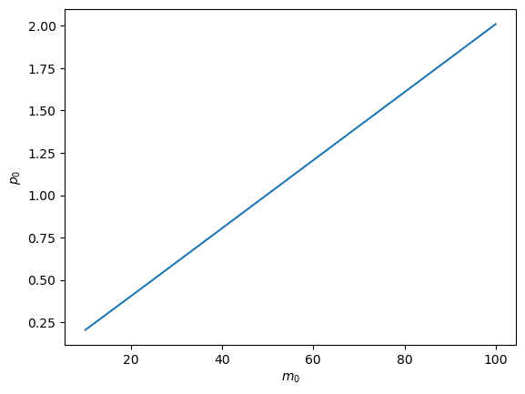
Let’s look at how price level \(p_0\) in the stationary \(R_u\) equilibrium depends on the initial money supply \(m_0\).
Notice that the slope of \(p_0\) as a function of \(m_0\) is constant.
This outcome indicates that our model verifies a quantity theory of money outcome, something that Sargent and Wallace [Sargent and Wallace, 1981] purposefully built into their model to justify the adjective monetarist in their title.
m0_arr = np.arange(10, 110, 10)
plt.plot(m0_arr, [compute_fixed_point(m0, 1, msm) for m0 in m0_arr])

plt.ylabel('$p_0$')
plt.xlabel('$m_0$')

plt.show()
Now let’s write and implement code that lets us experiment with the time \(0\) open market operation described earlier.
def simulate(m0, model, length=15, p0_guess=1):

    # unpack parameters
    γ1, γ2, g = model.γ1, model.γ2, model.g
    R_tilde = model.R_tilde
    m0_check, Bm1_check = model.m0_check, model.Bm1_check
    T = model.T

    # (pt, mt, bt, Rt)
    paths = np.empty((4, length))

    # open market operation
    p0 = compute_fixed_point(m0, 1, model)
    Bm1 = 1 / (p0 * R_tilde) * (m0_check - m0) + Bm1_check
    BTm1 = R_tilde ** T * Bm1 + ((1 - R_tilde ** T) / (1 - R_tilde)) * g
    g_bar = g + (R_tilde - 1) * BTm1
    Ru = np.roots((-γ1, γ1 + γ2 - g_bar, -γ2)).max()

    λ = γ2 / γ1

    # t = 0
    paths[0, 0] = p0
    paths[1, 0] = m0

    # 1 <= t <= T
    for t in range(1, T+1, 1):
        paths[0, t] = (1 / γ1) * m0 * \
                      ((1 - λ ** (T - t)) / (1 - λ)
                       + (λ ** (T - t) / (Ru - λ)))
        paths[1, t] = m0

    # t > T
    for t in range(T+1, length):
        paths[0, t] = paths[0, t-1] / Ru
        paths[1, t] = paths[1, t-1] + paths[0, t] * g_bar

    # Rt = pt / pt+1
    paths[3, :T] = paths[0, :T] / paths[0, 1:T+1]
    paths[3, T:] = Ru

    # bt = γ1 - γ2 / Rt
    paths[2, :] = γ1 - γ2 / paths[3, :]

    return paths
def plot_path(m0_arr, model, length=15):

    fig, axs = plt.subplots(2, 2, figsize=(8, 5))
    titles = ['$p_t$', '$m_t$', '$b_t$', '$R_t$']

    for m0 in m0_arr:
        paths = simulate(m0, model, length=length)
        for i, ax in enumerate(axs.flat):
            ax.plot(paths[i])
            ax.set_title(titles[i])

    axs[0, 1].hlines(model.m0_check, 0, length, color='r', linestyle='--')
    axs[0, 1].text(length * 0.8, model.m0_check * 0.9, r'$\check{m}_0$')
    plt.show()
plot_path([80, 100], msm)
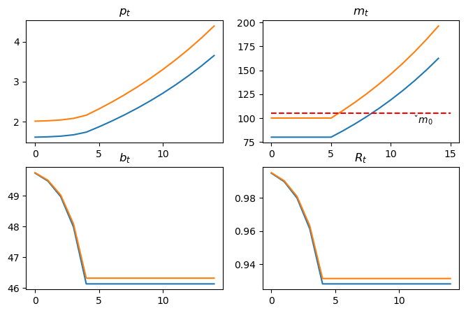
Fig. 31.1 Unpleasant Arithmetic#
Fig. 31.1 summarizes outcomes of two experiments that convey messages of Sargent and Wallace [Sargent and Wallace, 1981].
An open market operation that reduces the supply of money at time \(t=0\) reduces the price level at time \(t=0\)
The lower is the post-open-market-operation money supply at time \(0\), lower is the price level at time \(0\).
An open market operation that reduces the post open market operation money supply at time \(0\) also lowers the rate of return on money \(R_u\) at times \(t \geq T\) because it brings a higher gross of interest government deficit that must be financed by printing money (i.e., levying an inflation tax) at time \(t \geq T\).
\(R\) is important in the context of maintaining monetary stability and addressing the consequences of increased inflation due to government deficits. Thus, a larger \(R\) might be chosen to mitigate the negative impacts on the real rate of return caused by inflation.
31.9. Exercises#
Exercise 31.1
How the length of the tight-money period \(T\) amplifies unpleasant arithmetic.
The lecture shows that a central bank open-market operation that reduces \(m_0\) at \(t = 0\) lowers the price level immediately but forces a higher post-\(T\) deficit \(\bar g\) and therefore a lower rate of return \(R_u\) (higher inflation) forever after.
The same mechanism operates as \(T\) grows: holding \(m_0 = 100\) fixed, a longer period of bond-financed deficits accumulates more interest-bearing debt \(B_{T-1}\) that must eventually be serviced by printing money.
Fix \(m_0 = 100\) and vary \(T \in \{1, 3, 5, 10, 20\}\). For each \(T\):
a. Use simulate to obtain the stationary post-\(T\) rate of return
\(R_u\) (it equals paths[3, T]).
b. Compute the post-\(T\) government deficit \(\bar g = g + (\tilde R - 1) B_{T-1}\) directly from the model parameters and the fixed-point \(p_0\).
c. Plot \(R_u\) and \(\bar g\) against \(T\) on side-by-side panels and explain why \(R_u\) falls and \(\bar g\) rises as \(T\) increases.
Solution to Exercise 31.1
m0 = 100
T_values = [1, 3, 5, 10, 20]

R_u_list  = []
g_bar_list = []

for T_val in T_values:
    model_T = create_model(T=T_val)
    # equilibrium price level
    p0 = compute_fixed_point(m0, 1, model_T)
    # open-market operation creates bonds
    Bm1   = (1 / (p0 * model_T.R_tilde)) * (model_T.m0_check - m0) \
            + model_T.Bm1_check
    BTm1  = (model_T.R_tilde ** T_val * Bm1
             + (1 - model_T.R_tilde ** T_val) / (1 - model_T.R_tilde) * model_T.g)
    g_bar = model_T.g + (model_T.R_tilde - 1) * BTm1
    g_bar_list.append(g_bar)
    # post-T rate of return from simulate
    paths = simulate(m0, model_T, length=T_val + 3)
    R_u_list.append(paths[3, T_val])

fig, axes = plt.subplots(1, 2, figsize=(10, 4))

axes[0].plot(T_values, R_u_list, marker='o')
axes[0].set_xlabel('$T$')
axes[0].set_ylabel('$R_u$  (post-$T$ rate of return)')
axes[0].set_title('Longer tight-money period lowers $R_u$')

axes[1].plot(T_values, g_bar_list, marker='o', color='tab:orange')
axes[1].set_xlabel('$T$')
axes[1].set_ylabel(r'$\bar{g}$  (post-$T$ deficit)')
axes[1].set_title('Longer tight-money period raises $\\bar{g}$')

plt.tight_layout()
plt.show()

print(f"\n{'T':>4}  {'g_bar':>8}  {'R_u':>8}")
print('-' * 26)
for T_val, g_b, Ru in zip(T_values, g_bar_list, R_u_list):
    print(f"{T_val:>4}  {g_b:>8.4f}  {Ru:>8.4f}")
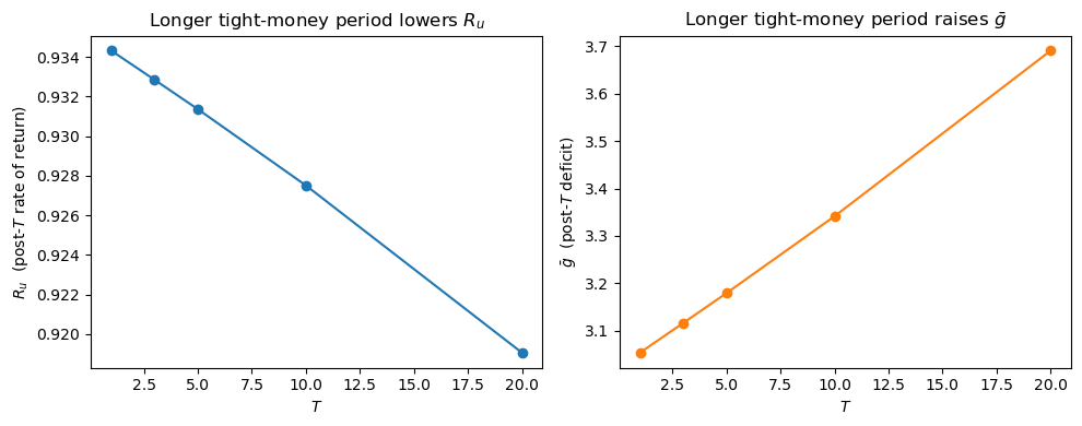
   T     g_bar       R_u
--------------------------
   1    3.0532    0.9343
   3    3.1159    0.9328
   5    3.1789    0.9314
  10    3.3412    0.9275
  20    3.6908    0.9191
Each additional period that \(m_t\) is held fixed forces the government to roll over its bonds at gross rate \(\tilde R > 1\), compounding the stock \(B_{T-1}\) and therefore raising \(\bar g\).
A higher \(\bar g\) sits further up the seigniorage Laffer curve, requiring a lower \(R_u\), or higher inflation tax rate.
This is the core mechanism of “unpleasant monetarist arithmetic”: tighter money today makes the long-run inflation rate higher, not lower.
Exercise 31.2
The fiscal limit: how large can \(T\) be?
The post-\(T\) deficit \(\bar g\) must be financeable by the inflation tax, which means it cannot exceed the maximum seigniorage revenue \(g_{\rm max} = S(\bar R_{\rm max})\) from the Laffer curve.
With \(m_0 = 100\) and the default parameters, find the fiscal limit \(T^*\): the largest integer \(T\) for which a feasible stationary equilibrium still exists after time \(T\) (i.e., \(\bar g \leq g_{\rm max}\)).
a. Compute \(g_{\rm max} = (\gamma_1 + \gamma_2) - \gamma_2/\bar R_{\rm max} - \gamma_1 \bar R_{\rm max}\) where \(\bar R_{\rm max} = \sqrt{\gamma_2/\gamma_1}\).
b. For \(T = 1, 2, \ldots, 150\), compute \(\bar g(T)\) as in Exercise 31.1.
Plot $\bar g(T)$ and $g_{\rm max}$ on the same axes and shade the infeasible region.
c. Identify \(T^*\), print \(\bar g\) at \(T^*\), and verify that no feasible real fixed point exists at \(T^* + 1\).
Solution to Exercise 31.2
γ1, γ2 = msm.γ1, msm.γ2

# Part a: Laffer-curve peak
R_max   = np.sqrt(γ2 / γ1)
g_max   = (γ1 + γ2) - γ2 / R_max - γ1 * R_max
print(f"R_max  = {R_max:.4f}")
print(f"g_max  = {g_max:.4f}")

# Part b: g_bar for T = 1 ... 150
m0 = 100
T_candidates = np.arange(1, 151)

def S_with_g_bar(p0, m0, model):
    γ1, γ2, g = model.γ1, model.γ2, model.g
    R_tilde = model.R_tilde
    m0_check, Bm1_check = model.m0_check, model.Bm1_check
    T = model.T

    Bm1 = 1 / (p0 * R_tilde) * (m0_check - m0) + Bm1_check
    BTm1 = (R_tilde ** T * Bm1
            + ((1 - R_tilde ** T) / (1 - R_tilde)) * g)
    g_bar = g + (R_tilde - 1) * BTm1

    disc = (γ1 + γ2 - g_bar)**2 - 4 * γ1 * γ2
    if disc < 0:
        return np.nan, np.nan, False

    Ru = ((γ1 + γ2 - g_bar) + np.sqrt(disc)) / (2 * γ1)
    λ = γ2 / γ1
    p0_new = (1 / γ1) * m0 * (
        (1 - λ ** T) / (1 - λ) + λ ** T / (Ru - λ))

    return p0_new, g_bar, True

def compute_fixed_point_and_g_bar(T_val, m0, p0_guess=1,
                                  θ=0.5, tol=1e-6, max_iter=10_000):
    model_T = create_model(T=int(T_val))
    p0 = p0_guess

    for _ in range(max_iter):
        p0_new, g_bar, real_roots = S_with_g_bar(p0, m0, model_T)
        if not real_roots:
            return np.nan, np.nan, False

        p0_next = (1 - θ) * p0_new + θ * p0
        if np.abs(p0_next - p0) < tol:
            _, g_bar, real_roots = S_with_g_bar(p0_next, m0, model_T)
            return p0_next, g_bar, real_roots

        p0 = p0_next

    return np.nan, np.nan, False

g_bar_arr = np.full(len(T_candidates), np.nan)
p0_guess = 1

for i, T_val in enumerate(T_candidates):
    p0_star, g_bar, real_roots = compute_fixed_point_and_g_bar(
        T_val, m0, p0_guess=p0_guess)
    if real_roots:
        g_bar_arr[i] = g_bar
        p0_guess = p0_star

finite = np.isfinite(g_bar_arr)
feasible = finite & (g_bar_arr <= g_max)

fig, ax = plt.subplots()
ax.plot(T_candidates[finite], g_bar_arr[finite], label=r'$\bar{g}(T)$')
ax.axhline(g_max, color='red', linestyle='--',
           label=f'$g_{{\\rm max}} = {g_max:.2f}$')
if np.any(feasible):
    T_star = T_candidates[feasible][-1]
    ax.axvspan(T_star + 1, T_candidates[-1], alpha=0.15, color='red',
               label='infeasible region')
ax.set_xlabel('$T$')
ax.set_ylabel(r'post-$T$ deficit $\bar{g}$')
ax.set_title('Fiscal limit: $\\bar{g}(T)$ vs Laffer-curve maximum')
ax.legend()
plt.tight_layout()
plt.show()

# Part c: fiscal limit T*
p0_next, g_bar_next, real_next = compute_fixed_point_and_g_bar(
    T_star + 1, m0, p0_guess=p0_guess)

print(f"\nFiscal limit T* = {T_star}")
print(f"  g_bar(T*)   = {g_bar_arr[T_star - 1]:.4f}  <=  g_max = {g_max:.4f}")
print(f"  Feasible real fixed point at T*+1 = {T_star + 1}: {real_next}")
R_max  = 0.7071
g_max  = 8.5786

Fiscal limit T* = 104
  g_bar(T*)   = 8.5136  <=  g_max = 8.5786
  Feasible real fixed point at T*+1 = 105: False
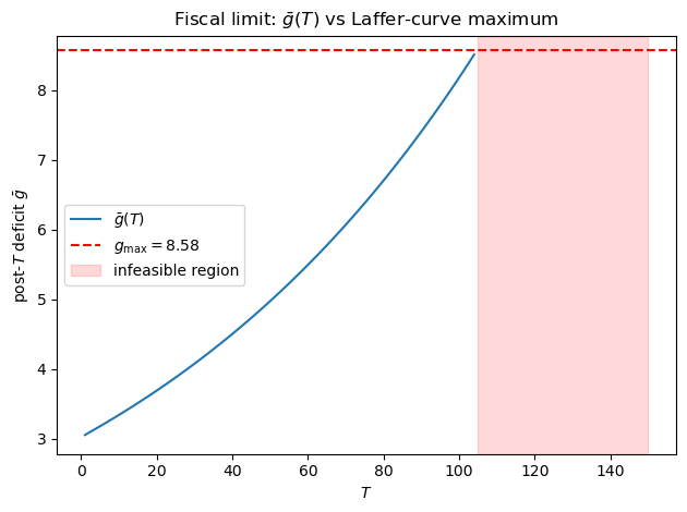
Beyond \(T^*\), the accumulated bond debt \(B_{T-1}\) is so large that the implied \(\bar g\) exceeds the peak of the seigniorage Laffer curve.
No matter how high the government sets the inflation tax rate, it cannot raise enough revenue to service that debt.
The fiscal limit is therefore a hard constraint on how long a tight-money policy can be pursued before the underlying fiscal arithmetic becomes incoherent.