15. Introduction to Bayesian Methods#
15.1. Overview#
In this lecture we study one of the most important ideas in statistics: how to update our beliefs about an unknown quantity as new data arrives.
The technique we will use is called Bayesian updating, named after Thomas Bayes.
We start with a belief about some unknown number.
As we observe data, we revise that belief in a way that is mathematically precise.
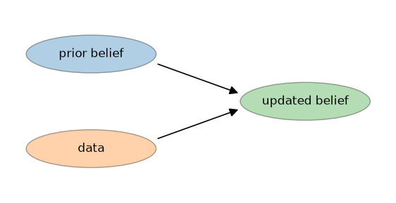
The figure below illustrates the idea: we combine a prior belief with observed data to arrive at an updated belief.
We will develop these ideas through an example drawn from development finance: estimating the default rate on a new type of loan.
Along the way we will meet conditional probability, Bayes’ law, the Bernoulli and binomial distributions, and the beta distribution.
Let’s begin by importing the libraries we need.
import numpy as np
import matplotlib.pyplot as plt
from matplotlib.lines import Line2D
from scipy.stats import beta, binom
15.2. Conditional probability#
Before we can talk about updating beliefs, we need to recall the idea of conditional probability.
15.2.1. Definition#
Suppose \(A\) and \(B\) are two events with \(P(B) > 0\).
The probability of \(A\) given that \(B\) has occurred is written \(P(A \mid B)\) and defined by
Here \(A \cap B\) is the event that both \(A\) and \(B\) occur.
The intuition is that learning \(B\) has occurred restricts us to the world in which \(B\) is true.
Within that restricted world, we ask how likely \(A\) is.
15.2.2. Example: risky borrowing#
A bank classifies its borrowers as either low risk or high risk.
Among all borrowers, 80% are low risk and 20% are high risk.
The conditional default probabilities are:
low-risk borrowers: 0.05
high-risk borrowers: 0.40
Suppose we pick a borrower at random and find that they defaulted.
What is the probability that the borrower was high risk?
Let \(H = \) high risk, \(L = \) low risk and \(D = \) default.
We know that \(P(H) = 0.2\), \(P(L) = 0.8\), \(P(D \mid H) = 0.40\) and \(P(D \mid L) = 0.05\).
The probability that a borrower is both high risk and defaults is
The overall probability of default can be computed from the law of total probability:
Applying (15.1), we get
So observing a default raises our assessment that the borrower is high risk from 20% to about 67%.
15.2.3. Bayes’ law#
The last computation was, in fact, a typical Bayesian calculation.
Let’s clarify further by returning to a setting with two abstract events \(A\) and \(B\).
Notice that the event \(A \cap B\) (both \(A\) and \(B\) occur) is the same as \(B \cap A\).
Hence, applying definition (15.1) two ways, we have
Dividing through by \(P(B)\) gives Bayes’ law:
In this setting, we call
\(P(A)\) the prior — our belief about \(A\) before seeing data,
\(P(B \mid A)\) the likelihood — how probable the data \(B\) is when \(A\) is true, and
\(P(A \mid B)\) the posterior — our updated belief about \(A\) after seeing \(B\).
The denominator \(P(B)\) is a normalizing constant that makes the posterior probabilities sum to one.
Example 15.1
The borrower calculation we completed above was an application of Bayes’ law with \(A = H\) and \(B = D\).
Bayes’ law tells us how to convert \(P(D \mid H)\), which was assumed to be known, into \(P(H \mid D)\), which we want.
15.3. A microloan default problem#
Now we turn to our main example.
A development bank is entering a new lending market — say, smallholder farmers in a region where no historical lending data exists.
The bank makes a series of small loans (microloans).
Each loan either defaults or is repaid.
We encode the outcome of loan \(i\) as a random variable \(Y_i\), where
Let \(\theta\) be the probability that any given loan defaults.
We assume that, given \(\theta\), the outcomes \(Y_1, Y_2, \ldots\) are independent draws with
A random variable of this form is called a Bernoulli random variable with parameter \(\theta\).
The catch is that the bank does not know \(\theta\).
Since the market is new, \(\theta\) is uncertain.
At the same time, the bank has experience in similar markets, so it does not start from total ignorance.
The Bayesian approach is to treat \(\theta\) as a random quantity and describe our beliefs about it with a probability density \(\pi\) on the interval \([0, 1]\).
This density is called the prior.
One possible option for \(\pi\) is to use a beta distribution, whose density on \([0,1]\) is
for parameters \(a > 0\) and \(b > 0\).
The denominator \(B(a, b)\) is called the beta function, and it is simply the constant that makes the density integrate to one.
For our purposes the important part is the shape, \(\theta^{a-1}(1-\theta)^{b-1}\), which is all that depends on \(\theta\).
One nice property of the beta distribution is that, by varying \(a\) and \(b\), we can represent a wide range of beliefs.
The four examples below range from “no idea at all” to at least some opinion as to whether \(\theta\) is likely to take a low or high value.
θ_grid = np.linspace(0, 1, 500)
plot_grid = np.linspace(0.001, 0.999, 500)   # avoids the spikes at the endpoints
params = [(0.5, 0.5), (1, 1), (2, 5), (8, 3)]

fig, axes = plt.subplots(2, 2, figsize=(10, 6))
for (a, b), ax in zip(params, axes.flatten()):
    ax.plot(plot_grid, beta.pdf(plot_grid, a, b), lw=2)
    ax.set_title(f"Beta({a}, {b})")
    ax.set_xlabel(r"$\theta$")
fig.tight_layout()
plt.show()
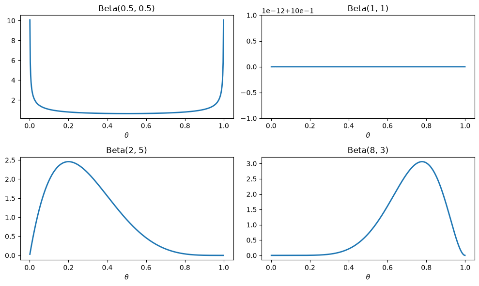
The shapes are strikingly different.
\(\text{Beta}(1, 1)\) is flat — it expresses complete ignorance, treating every default rate as equally likely.
\(\text{Beta}(0.5, 0.5)\) piles weight near 0 and 1, a belief that the market is probably either very safe or very risky.
\(\text{Beta}(2, 5)\) leans toward low default rates, while \(\text{Beta}(8, 3)\) leans toward high ones.
15.4. A one-step update#
Now suppose the bank observes the outcome of a single loan.
Call this outcome \(y \in \{0, 1\}\).
We want to update the prior \(\pi(\theta)\) into a posterior \(\pi(\theta \mid y)\).
The probability of \(y\) given \(\theta\) is
This formula (which is called the Bernoulli distribution) gives us the right numbers:
The default outcome \(y = 1\) yields \(\theta^1 (1-\theta)^0 = \theta\), the probability of a default.
The repayment outcome \(y = 0\) yields \(\theta^0 (1-\theta)^1 = 1 - \theta\), the probability of repayment.
Bayes’ law for a continuous parameter takes the form
This is the exact analogue of (15.2).
The numerator is likelihood times prior.
The denominator is an integral that sums the numerator over all possible values of \(\theta\), ensuring the posterior integrates to one.
Substituting the Bernoulli likelihood (15.3) gives our complete one-step update rule:
This rule is valid for any \(\theta\).
Hence we can think of it as taking any prior density \(\pi(\cdot)\) and any single observation \(y\) and converting it into the posterior density \(\pi(\cdot \mid y)\).
15.5. Computing the update numerically#
How can we compute the posterior density?
15.5.1. Prior#
First let’s set up the prior.
For our development bank we will begin with the prior \(\pi = \text{Beta}(2, 5)\).
a_0, b_0 = 2, 5

def pi(θ):
    return beta.pdf(θ, a_0, b_0)
This prior was shown above.
It puts most of its weight on default rates below 0.5, with a peak around 0.2, reflecting cautious optimism (most borrowers don’t default) together with significant uncertainty.
15.5.2. Normalizing constant#
Next we need to compute the constant in the denominator of (15.4), which is the integrated likelihood times the prior:
One general approach is to compute \(c(y)\) numerically, using a technique such as the trapezoidal rule.
The idea of the trapezoidal rule is to
fix a grid of points across \([0, 1]\),
join neighboring grid points by straight lines, and
sum the areas of the resulting trapezoids.
The figure below illustrates this for the integrand \(p(y \mid \theta)\, \pi(\theta)\) with \(y = 1\), using a coarse grid so the trapezoids are visible.
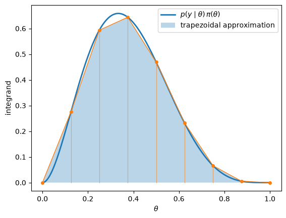
The finer the grid, the closer the shaded region gets to the true area under the curve.
The function below uses this method to compute an approximation of \(c(y)\).
def normalizing_constant(y):
    "Compute the denominator of Bayes' law: likelihood times prior, integrated."
    t_grid = np.linspace(0, 1, 100)  # linear grid of 100 points
    likelihood_vals = t_grid**y * (1 - t_grid)**(1 - y)
    prior_vals = pi(t_grid)
    integrand = likelihood_vals * prior_vals
    return np.trapezoid(integrand, t_grid)
15.5.3. Calculating the posterior#
The second step divides the (unnormalized) product of likelihood and prior by this constant.
The result is the posterior density, evaluated on the grid.
def update(y, θ_grid):
    """
    Compute posterior values pi(θ, y) on the set of grid points θ_grid
    after observing outcome y.
    """
    likelihood_vals = θ_grid**y * (1 - θ_grid)**(1 - y)
    prior_vals = pi(θ_grid)
    return likelihood_vals * prior_vals / normalizing_constant(y)
Let’s start from our Beta(2, 5) prior and suppose that we observe a single default (\(y = 1\)).
θ_grid = np.linspace(0, 1, 500)
prior_vals = pi(θ_grid)
posterior_vals = update(y=1, θ_grid=θ_grid)

fig, ax = plt.subplots()
ax.plot(θ_grid, prior_vals, lw=2, label="prior")
ax.plot(θ_grid, posterior_vals, lw=2, label="posterior after one default")
ax.set_xlabel(r"$\theta$")
ax.set_ylabel("density")
ax.legend()
plt.show()
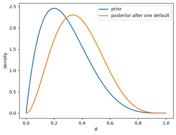
Observing a default shifts the posterior to the right, toward higher default probabilities.
This makes sense: a default is evidence that \(\theta\) might be larger than we thought.
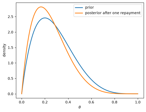
If instead the loan had been repaid, the posterior would shift left.
posterior_repaid = update(y=0, θ_grid=θ_grid)

fig, ax = plt.subplots()
ax.plot(θ_grid, prior_vals, lw=2, label="prior")
ax.plot(θ_grid, posterior_repaid, lw=2, label="posterior after one repayment")
ax.set_xlabel(r"$\theta$")
ax.set_ylabel("density")
ax.legend()
plt.show()
15.6. Iterating the update#
Here is a key observation: the posterior after one step is itself a perfectly good prior for the next step.
So we can repeat the update as each new loan resolves.
Starting from a prior \(\pi_0\), observing \(Y_1\) gives a posterior \(\pi_1\).
Treating \(\pi_1\) as the new prior and observing \(Y_2\) gives \(\pi_2\), and so on.
This produces a sequence of densities \(\pi_0, \pi_1, \pi_2, \ldots\) that captures our evolving beliefs.
Let’s simulate a stream of loan outcomes and watch the beliefs evolve.
We will generate data from a “true” default rate \(\theta^* = 0.15\), which the bank does not know.
θ_true = 0.15
n = 100
rng = np.random.default_rng(seed=42)
# Generate n draws from the Bernoulli distribution with θ = θ_true
outcomes = (rng.random(n) < θ_true).astype(int)
Now we iterate the grid update over these outcomes, recording the posterior at a sequence of stages and showing each in its own panel.
snapshots = [0, 1, 2, 3, 5, 8, 12, 16, 20]   # 0 = prior

# Iterate the grid update, saving the density at each snapshot
current_vals = pi(θ_grid)
saved = {0: current_vals.copy()}
for i in range(1, max(snapshots) + 1):
    y = outcomes[i - 1]
    likelihood_vals = θ_grid**y * (1 - θ_grid)**(1 - y)
    current_vals = likelihood_vals * current_vals
    current_vals /= np.trapezoid(current_vals, θ_grid)
    if i in snapshots:
        saved[i] = current_vals.copy()

# Use a common y-axis so the concentration over time is visible
y_max = max(vals.max() for vals in saved.values())

fig, axes = plt.subplots(3, 3, figsize=(6.2, 6.2), sharex=True, sharey=True)
for ax, k in zip(axes.flatten(), snapshots):
    ax.fill_between(θ_grid, saved[k], color='C0', alpha=0.3)
    ax.plot(θ_grid, saved[k], color='k', lw=1)
    ax.axvline(θ_true, color='k', ls=':', lw=1)
    ax.set_title("prior" if k == 0 else f"{k} loans", fontsize=10)
    ax.set_ylim(0, y_max * 1.05)
    ax.set_box_aspect(1)             # force each panel to be square
for ax in axes[-1, :]:
    ax.set_xlabel(r"$\theta$")
fig.tight_layout()
plt.show()
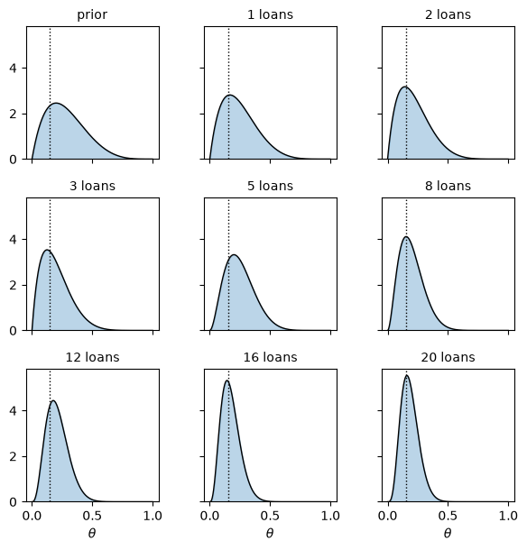
Two things stand out.
First, the posterior concentrates around the true value \(\theta^* = 0.15\) as more loans resolve.
Second, the posterior becomes tighter — our uncertainty about \(\theta\) steadily shrinks.
Early on, the prior has a strong influence on our beliefs.
As data accumulates, that influence fades and the data takes over.
15.7. Further observations#
Let’s make two additional observations regarding the model described above.
The first shows that we can do the update steps above with pencil and paper in the special case of a beta prior.
The second observation concerns batch updating.
15.7.1. A closed form: the beta prior#
The numerical updating rule provided above always works, regardless of our choice of prior.
But in the beta case we get a nice analytical approach as well.
Recall that this prior is proportional to \(\theta^{a-1}(1-\theta)^{b-1}\).
When we multiply this expression by the Bernoulli likelihood \(\theta^{y}(1-\theta)^{1-y}\), we get
The right-hand side has the form of another beta density.
So if the prior is \(\text{Beta}(a, b)\), the posterior is again a beta distribution — with updated parameters.
We say that the beta distribution is a conjugate prior for the Bernoulli likelihood.
The update rule for the parameters is very simple:
a default (\(y = 1\)) sends \((a, b) \mapsto (a + 1,\, b)\),
a repayment (\(y = 0\)) sends \((a, b) \mapsto (a,\, b + 1)\).
Let’s verify that this closed form agrees with our numerical computation.
We overlay the analytical \(\text{Beta}(a_0 + 1, b_0)\) posterior on the grid posterior after one default.
closed_form = beta.pdf(θ_grid, a_0 + 1, b_0)

fig, ax = plt.subplots()
ax.plot(θ_grid, posterior_vals, lw=4, alpha=0.5, label="numerical posterior")
ax.plot(θ_grid, closed_form, ls='--', lw=2, label=f"Beta({a_0 + 1}, {b_0})")
ax.set_xlabel(r"$\theta$")
ax.set_ylabel("density")
ax.legend()
plt.show()
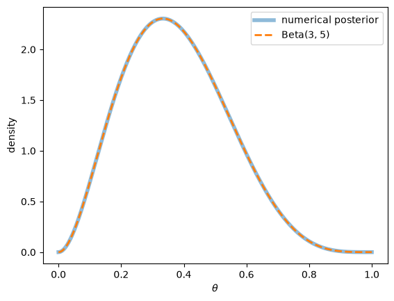
The two curves lie exactly on top of one another, confirming that our numerics and the closed form agree.
15.7.2. The batch update via the binomial likelihood#
There is a second, equally natural way to think about the problem of belief updating given loan outcome data.
Instead of processing outcomes one at a time, suppose we wait and observe all \(n\) outcomes \(Y_1, \ldots, Y_n\) together.
Then we update directly from the prior \(\pi_0\) to the posterior \(\pi_n\) in a single step.
Let the total number of defaults be given by
The probability of observing exactly \(k\) defaults out of \(n\) loans is given by the binomial distribution:
Bayes’ law then gives the one-shot update
With a \(\text{Beta}(a, b)\) prior, conjugacy again gives a clean closed form.
The binomial likelihood is proportional to \(\theta^{k}(1-\theta)^{n-k}\), so the posterior is
In words: add the number of defaults to \(a\), and add the number of repayments to \(b\).
15.8. Sequential and batch updates agree#
We now have two routes from prior to posterior.
One processes the \(n\) outcomes one at a time; the other processes them all at once.
Reassuringly, they give exactly the same answer.
We can see why with a short algebraic argument.
The likelihood of the full sequence \(Y_1, \ldots, Y_n\), for given \(\theta\), is the product of the individual Bernoulli likelihoods:
This is identical to the binomial likelihood (15.6), except for the factor \(\binom{n}{k}\).
But \(\binom{n}{k}\) does not depend on \(\theta\), so it cancels between the numerator and denominator when we normalize.
Hence the two posteriors are equal.
Note
It might appear that the sequential update never used the assumption that the outcomes are independent, while the batch update clearly did.
In fact both rely on it.
The honest update at step \(i\) conditions on everything seen so far:
When we replace \(p(Y_i \mid \theta, Y_1, \ldots, Y_{i-1})\) by the single-outcome likelihood \(p(Y_i \mid \theta)\), we are assuming that, given \(\theta\), the new outcome is independent of the past.
This is exactly the conditional independence that lets the batch likelihood factor into a product.
So the assumption is doing the same work in both routes — it is just hidden in the sequential one.
15.9. From posterior to loan pricing#
Why does any of this matter for the bank?
The whole point of estimating \(\theta\) is to make better lending decisions.
Let’s discuss how this can be done.
15.9.1. Expected loss#
Suppose each loan has size 1, and the bank loses the full amount when a loan defaults.
Then the expected loss on a new loan is just the probability of default.
Given the data, our best estimate of that probability is the posterior mean.
Recall that the posterior is \(\text{Beta}(a + k,\ b + n - k)\).
The mean of a beta distribution \(\text{Beta}(\alpha, \beta)\) is \(\alpha / (\alpha + \beta)\), so here
This is the number the bank should plug into its pricing: to break even, the interest rate must at least cover the expected loss.
Let’s track how the expected loss, and our uncertainty about it, evolve as loans resolve.
cum_defaults = np.cumsum(outcomes)
loans = np.arange(1, n + 1)

a_n = a_0 + cum_defaults
b_n = b_0 + loans - cum_defaults

# Posterior mean at every n (vectorized); reused later for pricing
post_mean = a_n / (a_n + b_n)

# Draw the full posterior at a selection of sample sizes as violins
sample_points = [1, 5, 10, 20, 50, 100]
draw_rng = np.random.default_rng(12345)
samples = [beta.rvs(a_n[m - 1], b_n[m - 1], size=10_000, random_state=draw_rng)
           for m in sample_points]
means = [post_mean[m - 1] for m in sample_points]

fig, ax = plt.subplots()
positions = np.arange(len(sample_points))
ax.violinplot(samples, positions=positions,
              showmeans=False, showextrema=False)
ax.hlines(means, positions - 0.25, positions + 0.25, color='k', lw=3, zorder=3)
true_line = ax.axhline(θ_true, color='k', ls=':', lw=1)

# Use a short horizontal bar (not the hlines handle) for the mean in the legend
mean_proxy = Line2D([0], [0], color='k', lw=3)
ax.legend([mean_proxy, true_line],
          ["posterior mean (expected loss)", r"true $\theta^*$"])
ax.set_xticks(positions)
ax.set_xticklabels(sample_points)
ax.set_xlabel("number of loans observed")
ax.set_ylabel(r"$\theta$")
plt.show()
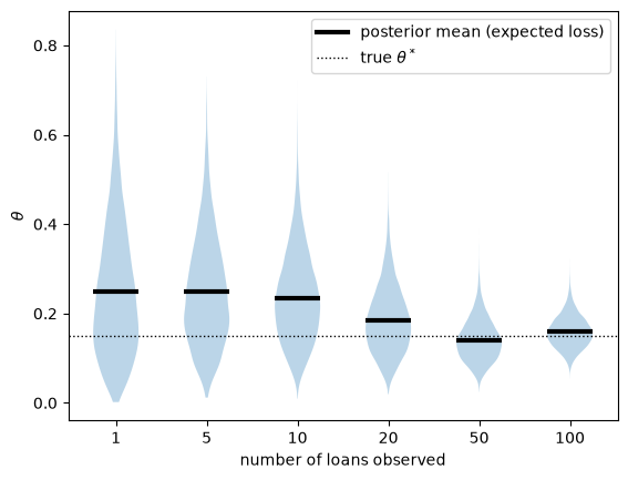
As the bank observes more loans, its estimate of the expected loss settles down near the true default rate.
At the same time, the violins narrow, showing that the posterior tightens around that estimate.
This is the practical payoff of Bayesian updating: the bank can price cautiously when data is scarce, and sharpen its pricing as experience accumulates.
15.9.2. The break-even interest rate#
Let’s turn the expected loss into an actual interest rate.
Consider a loan of size 1, carrying interest rate \(r\).
If the borrower repays, the bank receives \(1 + r\).
If the borrower defaults, the bank receives nothing.
Suppose the bank is risk neutral, faces no funding costs, and operates in a competitive market that drives expected profits to zero.
The zero-profit condition sets the expected repayment equal to the amount lent:
Solving for \(r\) gives the break-even interest rate
This rate has a clean interpretation: the expected interest income \((1 - \theta) r\) exactly equals the expected loss \(\theta\).
Of course the bank does not know \(\theta\).
Because the bank is risk neutral, only the mean of \(\theta\) enters the calculation, so it replaces \(\theta\) by its posterior mean \(\hat\theta = \mathbb{E}[\theta \mid \text{data}]\):
Let’s see how this break-even rate evolves as the loan book grows.
implied_rate = post_mean / (1 - post_mean)

fig, ax = plt.subplots()
ax.plot(loans, implied_rate, lw=2, label="break-even rate")
ax.axhline(θ_true / (1 - θ_true), color='k', ls=':',
           label=r"rate at true $\theta^*$")
ax.set_xlabel("number of loans observed")
ax.set_ylabel(r"interest rate $r$")
ax.legend()
plt.show()
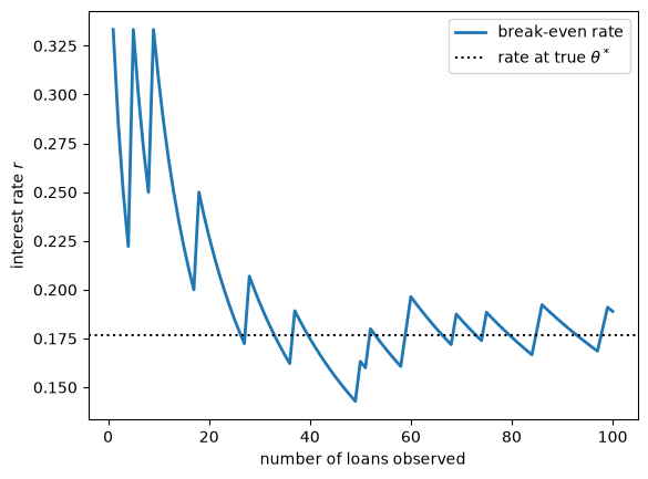
Early on, with little data, the rate reflects the prior and is somewhat unstable.
As loans resolve, it settles toward \(\theta^* / (1 - \theta^*) \approx 0.176\), the rate the bank would charge if it knew the true default probability.
15.10. Exercises#
Exercise 15.1
The prior matters a lot when data is scarce, but its influence should fade as data accumulates.
Illustrate this by repeating the iteration of the previous sections from two very different priors:
an optimistic prior \(\text{Beta}(2, 8)\), which expects a low default rate, and
a skeptical prior \(\text{Beta}(8, 2)\), which expects a high default rate.
Use the same simulated data (with \(\theta^* = 0.15\)) for both.
Plot the two posterior means as a function of the number of loans observed, and confirm that they converge as \(n\) grows.
Solution
We can use the conjugate update rule directly, since both priors are beta distributions.
priors = {"optimistic Beta(2, 8)": (2, 8),
          "skeptical Beta(8, 2)": (8, 2)}

cum_defaults = np.cumsum(outcomes)
loans = np.arange(1, n + 1)

fig, ax = plt.subplots()
for label, (a, b) in priors.items():
    a_seq = a + cum_defaults
    b_seq = b + loans - cum_defaults
    ax.plot(loans, a_seq / (a_seq + b_seq), lw=2, label=label)

ax.axhline(θ_true, color='k', ls=':', label=r"true $\theta^*$")
ax.set_xlabel("number of loans observed")
ax.set_ylabel("posterior mean")
ax.legend()
plt.show()
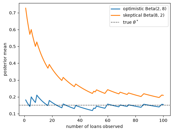
The two estimates start far apart, reflecting the disagreement between the priors.
As loans accumulate, both are pulled toward the true value \(\theta^* = 0.15\) and the gap between them shrinks.
With enough data, the choice of prior barely matters — the data dominates.
Exercise 15.2
Suppose the bank starts with a \(\text{Beta}(2, 5)\) prior and then observes 200 loans, of which 26 default.
Compute the posterior mean default rate.
Compute a 90% credible interval for \(\theta\) — an interval that contains \(\theta\) with posterior probability 0.90.
For the credible interval, use the 5th and 95th percentiles of the posterior, available via beta.ppf.
Solution
The posterior is \(\text{Beta}(a_0 + k,\ b_0 + n - k)\) with \(a_0 = 2\), \(b_0 = 5\), \(n = 200\) and \(k = 26\).
a_post = 2 + 26
b_post = 5 + (200 - 26)

post_mean = a_post / (a_post + b_post)
lower, upper = beta.ppf([0.05, 0.95], a_post, b_post)

print(f"Posterior: Beta({a_post}, {b_post})")
print(f"Posterior mean default rate: {post_mean:.4f}")
print(f"90% credible interval: ({lower:.4f}, {upper:.4f})")
Posterior: Beta(28, 179)
Posterior mean default rate: 0.1353
90% credible interval: (0.0984, 0.1762)
The bank’s best estimate of the default rate is about 13.5%, and it is 90% sure that the true rate lies within the reported interval.
These two numbers — a point estimate and a measure of uncertainty — are exactly what is needed to price the loans.