38. Linear Programming

In this lecture, we will need the following imports.

import numpy as np
from scipy.optimize import linprog
import matplotlib.pyplot as plt
from matplotlib.patches import Polygon

38.1. Overview

Linear programming problems either maximize or minimize a linear objective function subject to a set of linear equality and/or inequality constraints.

Linear programs come in pairs:

• an original primal problem, and

• an associated dual problem.

If a primal problem involves maximization, the dual problem involves minimization.

If a primal problem involves minimization, the dual problem involves maximization.

In this lecture we will

• present two example problems,

• describe a standard form that lets us hand any linear program to a black-box solver,

• solve both examples using SciPy, and

• study the dual problem and its economic interpretation in terms of shadow prices.

We will solve our linear programs with SciPy’s linprog function, which calls the high-performance HiGHS solver.

See also

In another lecture, we will employ the linear programming method to solve the optimal transport problem.

Let’s start with some examples of linear programming problems.

38.2. Example 1: production problem

This example was created by [Bertsimas, 1997].

Suppose that a factory can produce two goods called Product \(1\) and Product \(2\).

To produce each product requires both material and labor.

Selling each product generates revenue.

Required per unit material and labor inputs and revenues are shown in table below:

	Product 1	Product 2
Material	2	5
Labor	4	2
Revenue	3	4

30 units of material and 20 units of labor available.

A firm’s problem is to construct a production plan that uses its 30 units of materials and 20 units of labor to maximize its revenue.

Let \(x_i\) denote the quantity of Product \(i\) that the firm produces and \(z\) denote the total revenue.

This problem can be formulated as:

\[\begin{split} \begin{aligned} \max_{x_1,x_2} \ & z = 3 x_1 + 4 x_2 \\ \mbox{subject to } \ & 2 x_1 + 5 x_2 \le 30 \\ & 4 x_1 + 2 x_2 \le 20 \\ & x_1, x_2 \ge 0 \\ \end{aligned} \end{split}\]

We allow \(x_1\) and \(x_2\) to take any nonnegative real values.

If we instead required them to be whole numbers, the problem would become an integer program, which is typically much harder to solve.

Allowing real values keeps the feasible set convex, and that convexity is what makes linear programming so tractable.

38.2.1. A graphical solution

Because this problem has only two decision variables, we can solve it graphically.

The following graph illustrates the firm’s constraints and iso-revenue lines.

Iso-revenue lines show all the combinations of Product 1 and Product 2 that generate the same revenue.

Show source

Hide code cell source

fig, ax = plt.subplots()
# Draw constraint lines
ax.set_xlim(0,15)
ax.set_ylim(0,10)
x1 = np.linspace(0, 15)
ax.plot(x1, 6-0.4*x1, label="$2x_1 + 5x_2=30$")
ax.plot(x1, 10-2*x1, label="$4x_1 + 2x_2=20$")


# Draw the feasible region
feasible_set = Polygon(np.array([[0, 0],[0, 6],[2.5, 5],[5, 0]]), alpha=0.1)
ax.add_patch(feasible_set)

# Draw the objective function
ax.plot(x1, 3.875-0.75*x1, label="iso-revenue lines",color='k',linewidth=0.75)
ax.plot(x1, 5.375-0.75*x1, color='k',linewidth=0.75)
ax.plot(x1, 6.875-0.75*x1, color='k',linewidth=0.75)

# Draw the optimal solution
ax.plot(2.5, 5, ".", label="optimal solution")
ax.set_xlabel("$x_1$")
ax.set_ylabel("$x_2$")
ax.legend()

plt.show()

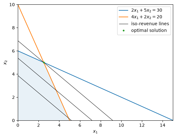
The blue region is the feasible set within which all constraints are satisfied.

Parallel black lines are iso-revenue lines.

The firm’s objective is to push the iso-revenue line as high as possible while remaining in the feasible set.

The intersection of the feasible set and the highest iso-revenue line delineates the optimal set.

In this example, the optimal set is the point \((2.5, 5)\), which generates revenue \(z = 3 \times 2.5 + 4 \times 5 = 27.5\).

This graphical method works nicely in two dimensions.

But it does not scale: with more than two or three decision variables we can no longer draw the feasible set.

Our next example has five decision variables, so we will need a systematic computational method.

38.3. Example 2: investment problem

We now consider a problem posed and solved by [Hu, 2018].

A mutual fund has \( \$ 100,000\) to be invested over a three-year horizon.

Three investment options are available:

1. Annuity: the fund can pay a same amount of new capital at the beginning of each of three years and receive a payoff of 130% of total capital invested at the end of the third year. Once the mutual fund decides to invest in this annuity, it has to keep investing in all subsequent years in the three year horizon.

2. Bank account: the fund can deposit any amount into a bank at the beginning of each year and receive its capital plus 6% interest at the end of that year. In addition, the mutual fund is permitted to borrow no more than $20,000 at the beginning of each year and is asked to pay back the amount borrowed plus 6% interest at the end of the year. The mutual fund can choose whether to deposit or borrow at the beginning of each year.

3. Corporate bond: At the beginning of the second year, a corporate bond becomes available. The fund can buy an amount that is no more than \( \$ \)50,000 of this bond at the beginning of the second year and at the end of the third year receive a payout of 130% of the amount invested in the bond.

The mutual fund’s objective is to maximize total payout that it owns at the end of the third year.

We can formulate this as a linear programming problem.

Let \(x_1\) be the amount of put in the annuity, \(x_2, x_3, x_4\) be bank deposit balances at the beginning of the three years, and \(x_5\) be the amount invested in the corporate bond.

When \(x_2, x_3, x_4\) are negative, it means that the mutual fund has borrowed from bank.

The table below shows the mutual fund’s decision variables together with the timing protocol described above:

	Year 1	Year 2	Year 3
Annuity	\(x_1\)	\(x_1\)	\(x_1\)
Bank account	\(x_2\)	\(x_3\)	\(x_4\)
Corporate bond	0	\(x_5\)	0

The mutual fund’s decision making proceeds according to the following timing protocol:

1. At the beginning of the first year, the mutual fund decides how much to invest in the annuity and how much to deposit in the bank. This decision is subject to the constraint:

   \[ x_1 + x_2 = 100,000 \]

2. At the beginning of the second year, the mutual fund has a bank balance of \(1.06 x_2\). It must keep \(x_1\) in the annuity. It can choose to put \(x_5\) into the corporate bond, and put \(x_3\) in the bank. These decisions are restricted by

   \[ x_1 + x_5 = 1.06 x_2 - x_3 \]

3. At the beginning of the third year, the mutual fund has a bank account balance equal to \(1.06 x_3\). It must again invest \(x_1\) in the annuity, leaving it with a bank account balance equal to \(x_4\). This situation is summarized by the restriction:

   \[ x_1 = 1.06 x_3 - x_4 \]

The mutual fund’s objective function, i.e., its wealth at the end of the third year is:

\[ 1.30 \cdot 3x_1 + 1.06 x_4 + 1.30 x_5 \]

Thus, the mutual fund confronts the linear program:

\[\begin{split} \begin{aligned} \max_{x} \ & 1.30 \cdot 3x_1 + 1.06 x_4 + 1.30 x_5 \\ \mbox{subject to } \ & x_1 + x_2 = 100,000\\ & x_1 - 1.06 x_2 + x_3 + x_5 = 0\\ & x_1 - 1.06 x_3 + x_4 = 0\\ & x_2 \ge -20,000\\ & x_3 \ge -20,000\\ & x_4 \ge -20,000\\ & x_5 \le 50,000\\ & x_j \ge 0, \quad j = 1,5\\ & x_j \ \text{unrestricted}, \quad j = 2,3,4\\ \end{aligned} \end{split}\]

This problem has five decision variables and three equality constraints, along with several bounds.

Unlike Example 1, we cannot represent it in a two-dimensional graph and read off the solution.

To solve problems like this we first cast them in a standard form and then hand them to a solver.

38.4. Standard form

For purposes of

• unifying linear programs that are initially stated in superficially different forms, and

• having a form that is convenient to put into black-box software packages,

it is useful to devote some effort to describe a standard form.

Our standard form is:

\[\begin{split} \begin{aligned} \min_{x} \ & c_1 x_1 + c_2 x_2 + \dots + c_n x_n \\ \mbox{subject to } \ & a_{11} x_1 + a_{12} x_2 + \dots + a_{1n} x_n = b_1 \\ & a_{21} x_1 + a_{22} x_2 + \dots + a_{2n} x_n = b_2 \\ & \quad \vdots \\ & a_{m1} x_1 + a_{m2} x_2 + \dots + a_{mn} x_n = b_m \\ & x_1, x_2, \dots, x_n \ge 0 \\ \end{aligned} \end{split}\]

Let

\[\begin{split} A = \begin{bmatrix} a_{11} & a_{12} & \dots & a_{1n} \\ a_{21} & a_{22} & \dots & a_{2n} \\ & & \vdots & \\ a_{m1} & a_{m2} & \dots & a_{mn} \\ \end{bmatrix}, \quad b = \begin{bmatrix} b_1 \\ b_2 \\ \vdots \\ b_m \\ \end{bmatrix}, \quad c = \begin{bmatrix} c_1 \\ c_2 \\ \vdots \\ c_n \\ \end{bmatrix}, \quad x = \begin{bmatrix} x_1 \\ x_2 \\ \vdots \\ x_n \\ \end{bmatrix}. \quad \end{split}\]

The standard form linear programming problem can be expressed concisely as:

(38.1)\[\begin{split} \begin{aligned} \min_{x} \ & c'x \\ \mbox{subject to } \ & Ax = b\\ & x \geq 0\\ \end{aligned} \end{split}\]

Here, \(Ax = b\) means that the \(i\)-th entry of \(Ax\) equals the \(i\)-th entry of \(b\) for every \(i\).

Similarly, \(x \geq 0\) means that \(x_j\) is greater than or equal to \(0\) for every \(j\).

38.4.1. Useful transformations

It is useful to know how to transform a problem that initially is not stated in the standard form into one that is.

By deploying the following steps, any linear programming problem can be transformed into an equivalent standard form linear programming problem.

1. Objective function: If a problem is originally a constrained maximization problem, we can construct a new objective function that is the additive inverse of the original objective function. The transformed problem is then a minimization problem.

2. Decision variables: Given a variable \(x_j\) satisfying \(x_j \le 0\), we can introduce a new variable \(x_j' = - x_j\) and substitute it into original problem. Given a free variable \(x_i\) with no restriction on its sign, we can introduce two new variables \(x_j^+\) and \(x_j^-\) satisfying \(x_j^+, x_j^- \ge 0\) and replace \(x_j\) by \(x_j^+ - x_j^-\).

3. Inequality constraints: Given an inequality constraint \(\sum_{j=1}^n a_{ij}x_j \le b_i\), we can introduce a new variable \(s_i\), called a slack variable that satisfies \(s_i \ge 0\) and replace the original constraint by \(\sum_{j=1}^n a_{ij}x_j + s_i = b_i\).

Let’s apply the above steps to the two examples described above.

38.4.2. Example 1: production problem

The original problem is:

\[\begin{split} \begin{aligned} \max_{x_1,x_2} \ & 3 x_1 + 4 x_2 \\ \mbox{subject to } \ & 2 x_1 + 5 x_2 \le 30 \\ & 4 x_1 + 2 x_2 \le 20 \\ & x_1, x_2 \ge 0 \\ \end{aligned} \end{split}\]

This problem is equivalent to the following problem with a standard form:

\[\begin{split} \begin{aligned} \min_{x_1,x_2} \ & -(3 x_1 + 4 x_2) \\ \mbox{subject to } \ & 2 x_1 + 5 x_2 + s_1 = 30 \\ & 4 x_1 + 2 x_2 + s_2 = 20 \\ & x_1, x_2, s_1, s_2 \ge 0 \\ \end{aligned} \end{split}\]

38.4.3. Example 2: investment problem

The original problem is:

\[\begin{split} \begin{aligned} \max_{x} \ & 1.30 \cdot 3x_1 + 1.06 x_4 + 1.30 x_5 \\ \mbox{subject to } \ & x_1 + x_2 = 100,000\\ & x_1 - 1.06 x_2 + x_3 + x_5 = 0\\ & x_1 - 1.06 x_3 + x_4 = 0\\ & x_2 \ge -20,000\\ & x_3 \ge -20,000\\ & x_4 \ge -20,000\\ & x_5 \le 50,000\\ & x_j \ge 0, \quad j = 1,5\\ & x_j \ \text{unrestricted}, \quad j = 2,3,4\\ \end{aligned} \end{split}\]

This problem is equivalent to the following problem with a standard form:

\[\begin{split} \begin{aligned} \min_{x} \ & -(1.30 \cdot 3x_1 + 1.06 x_4^+ - 1.06 x_4^- + 1.30 x_5) \\ \mbox{subject to } \ & x_1 + x_2^+ - x_2^- = 100,000\\ & x_1 - 1.06 (x_2^+ - x_2^-) + x_3^+ - x_3^- + x_5 = 0\\ & x_1 - 1.06 (x_3^+ - x_3^-) + x_4^+ - x_4^- = 0\\ & x_2^- - x_2^+ + s_1 = 20,000\\ & x_3^- - x_3^+ + s_2 = 20,000\\ & x_4^- - x_4^+ + s_3 = 20,000\\ & x_5 + s_4 = 50,000\\ & x_j \ge 0, \quad j = 1,5\\ & x_j^+, x_j^- \ge 0, \quad j = 2,3,4\\ & s_j \ge 0, \quad j = 1,2,3,4\\ \end{aligned} \end{split}\]

38.5. Computation: solving with SciPy

The package scipy.optimize provides a function linprog to solve linear programming problems with the form below:

\[\begin{split} \begin{aligned} \min_{x} \ & c' x \\ \mbox{subject to } \ & A_{ub}x \le b_{ub} \\ & A_{eq}x = b_{eq} \\ & l \le x \le u \\ \end{aligned} \end{split}\]

\(A_{eq}, b_{eq}\) denote the equality constraint matrix and vector, and \(A_{ub}, b_{ub}\) denote the inequality constraint matrix and vector.

Note

By default \(l = 0\) and \(u = \text{None}\) unless explicitly specified with the argument bounds.

Notice that we do not need to convert the problems to the standard form ourselves.

linprog accepts inequality constraints, equality constraints and variable bounds directly.

It is, however, helpful to understand the standard form, because it is what solvers use internally.

By default, linprog uses the highs method, which calls the high-performance HiGHS solver.

We use linprog as a black box: we describe the problem in terms of \(c\), \(A\) and \(b\), and the solver returns an optimal solution.

38.5.1. Example 1: production problem

Let’s solve Example 1 using SciPy.

Because linprog minimizes the objective, and our problem is a maximization, we pass \(-c\) and negate the result.

# Construct parameters
c_ex1 = np.array([3, 4])

# Inequality constraints
A_ex1 = np.array([[2, 5],
                  [4, 2]])
b_ex1 = np.array([30, 20])

Once we solve the problem, we can check whether the solver was successful in solving the problem using the boolean attribute success. If it’s successful, then the success attribute is set to True.

# Solve the problem
# we put a negative sign on the objective as linprog does minimization
res_ex1 = linprog(-c_ex1, A_ub=A_ex1, b_ub=b_ex1)

if res_ex1.success:
    # We use negative sign to get the optimal value (maximized value)
    print('Optimal Value:', -res_ex1.fun)
    print(f'(x1, x2): {res_ex1.x[0], res_ex1.x[1]}')
else:
    print('The problem does not have an optimal solution.')

Optimal Value: 27.5
(x1, x2): (np.float64(2.5), np.float64(5.0))

This confirms the answer we found graphically: produce \(2.5\) units of Product 1 and \(5\) units of Product 2, generating maximal revenue of \(27.5\).

The slack value returned by linprog is a one-dimensional NumPy array whose entries measure the difference \(b_{ub} - A_{ub}x\) for each inequality constraint.

res_ex1.slack

array([0., 0.])

Both slacks are zero, which tells us that both the material and labor constraints bind at the optimum.

See the official documentation for more details.

38.5.2. Example 2: investment problem

Now let’s solve the investment problem.

This time we use equality constraints A_eq, b_eq and supply bounds for each variable.

The bounds capture the borrowing limit (\(x_2, x_3, x_4 \ge -20{,}000\)) and the cap on the corporate bond (\(0 \le x_5 \le 50{,}000\)).

# Construct parameters
rate = 1.06

# Objective function parameters
c_ex2 = np.array([1.30*3, 0, 0, 1.06, 1.30])

# Equality constraints
A_ex2 = np.array([[1,  1,  0,  0,  0],
                  [1, -rate, 1, 0, 1],
                  [1, 0, -rate, 1, 0]])
b_ex2 = np.array([100_000, 0, 0])

# Bounds on decision variables
bounds_ex2 = [(  0,    None),
              (-20_000, None),
              (-20_000, None),
              (-20_000, None),
              (  0,   50_000)]

Let’s solve the problem and check the status using success attribute.

# Solve the problem
res_ex2 = linprog(-c_ex2, A_eq=A_ex2, b_eq=b_ex2,
                  bounds=bounds_ex2)

if res_ex2.success:
    # We use negative sign to get the optimal value (maximized value)
    print('Optimal Value:', -res_ex2.fun)
    x1_sol = round(res_ex2.x[0], 3)
    x2_sol = round(res_ex2.x[1], 3)
    x3_sol = round(res_ex2.x[2], 3)
    x4_sol = round(res_ex2.x[3], 3)
    x5_sol = round(res_ex2.x[4], 3)
    print(f'(x1, x2, x3, x4, x5): {x1_sol, x2_sol, x3_sol, x4_sol, x5_sol}')
else:
    print('The problem does not have an optimal solution.')

Optimal Value: 141018.24349792697
(x1, x2, x3, x4, x5): (np.float64(24927.755), np.float64(75072.245), np.float64(4648.825), np.float64(-20000.0), np.float64(50000.0))

SciPy tells us that the best investment strategy is:

1. At the beginning of the first year, the mutual fund should buy \( \$24,927.75\) of the annuity. Its bank account balance should be \( \$75,072.25\).

2. At the beginning of the second year, the mutual fund should buy \( \$50,000 \) of the corporate bond and keep investing in the annuity. Its bank account balance should be \( \$ 4,648.83\).

3. At the beginning of the third year, the mutual fund should borrow \( \$20,000\) from the bank and invest in the annuity.

4. At the end of the third year, the mutual fund will get payouts from the annuity and corporate bond and repay its loan from the bank. At the end it will own \( \$141,018.24 \), so that its total net rate of return over the three periods is \( 41.02\% \).

38.6. Duality

Every linear program, which we call the primal problem, has an associated linear program called its dual.

The dual problem provides valuable information about the primal, and its variables have an important economic interpretation as shadow prices.

Let’s develop these ideas using the production problem from Example 1.

38.6.1. The dual of the production problem

Recall the primal production problem:

\[\begin{split} \begin{aligned} \max_{x_1,x_2} \ & 3 x_1 + 4 x_2 \\ \mbox{subject to } \ & 2 x_1 + 5 x_2 \le 30 \\ & 4 x_1 + 2 x_2 \le 20 \\ & x_1, x_2 \ge 0 \\ \end{aligned} \end{split}\]

Imagine an outside investor who wants to buy all of the firm’s material and labor.

The investor must choose a price \(y_1\) for each unit of material and a price \(y_2\) for each unit of labor.

To persuade the firm to sell rather than produce, the prices must make each product at least as valuable sold as raw inputs as it is when turned into output.

Product 1 uses 2 units of material and 4 units of labor and earns revenue 3, so the investor needs

\[ 2 y_1 + 4 y_2 \ge 3 . \]

Product 2 uses 5 units of material and 2 units of labor and earns revenue 4, so the investor needs

\[ 5 y_1 + 2 y_2 \ge 4 . \]

Subject to these constraints, the investor wants to minimize the total amount paid for the firm’s 30 units of material and 20 units of labor.

This gives the dual problem:

\[\begin{split} \begin{aligned} \min_{y_1,y_2} \ & 30 y_1 + 20 y_2 \\ \mbox{subject to } \ & 2 y_1 + 4 y_2 \ge 3 \\ & 5 y_1 + 2 y_2 \ge 4 \\ & y_1, y_2 \ge 0 \\ \end{aligned} \end{split}\]

In general, the canonical primal-dual pair is

\[ \max_{x} \ c'x \ \text{ s.t. } \ Ax \le b, \ x \ge 0 \qquad \Longleftrightarrow \qquad \min_{y} \ b'y \ \text{ s.t. } \ A'y \ge c, \ y \ge 0 . \]

Notice that the primal has one variable per product and one constraint per resource, while the dual has one variable per resource and one constraint per product.

38.6.2. Solving the dual

Let’s solve the dual with linprog.

We rewrite the \(\ge\) constraints as \(\le\) constraints by multiplying them by \(-1\), since linprog expects inequalities in the form \(A_{ub} y \le b_{ub}\).

# Objective: minimize 30 y1 + 20 y2
b_dual = np.array([30, 20])

# Constraints A' y >= c  rewritten as -A' y <= -c
A_dual = np.array([[-2, -4],
                   [-5, -2]])
c_dual = np.array([-3, -4])

res_dual = linprog(b_dual, A_ub=A_dual, b_ub=c_dual)

print('Dual optimal value:', res_dual.fun)
print(f'(y1, y2): {res_dual.x[0], res_dual.x[1]}')

Dual optimal value: 27.5
(y1, y2): (np.float64(0.625), np.float64(0.43749999999999994))

The dual optimal value is \(27.5\) – exactly the primal optimal value.

This is no coincidence.

38.6.3. Weak and strong duality

For the canonical pair above, two key facts hold.

Weak duality: for any primal-feasible \(x\) and any dual-feasible \(y\) we have \(c'x \le b'y\).

So every dual-feasible point provides an upper bound on the primal maximum.

Strong duality: if either problem has an optimal solution, then so does the other, and their optimal values are equal.

Strong duality is why both linprog calls returned \(27.5\).

38.6.4. Shadow prices

The dual solution is \((y_1, y_2) = (0.625, 0.4375)\).

These numbers are the shadow prices of material and labor.

The shadow price of a resource measures how much the optimal revenue would rise if we had one more unit of that resource.

Let’s check this for material by re-solving the primal with the material constraint relaxed from \(30\) to \(31\).

b_relaxed = np.array([31, 20])
res_relaxed = linprog(-c_ex1, A_ub=A_ex1, b_ub=b_relaxed)

print('Revenue with 31 units of material:', -res_relaxed.fun)
print('Increase in revenue:', -res_relaxed.fun - (-res_ex1.fun))

Revenue with 31 units of material: 28.125
Increase in revenue: 0.625

The revenue rises by exactly \(0.625\), the shadow price of material.

In words, an extra unit of material is worth \(0.625\) to the firm, and an extra unit of labor is worth \(0.4375\).

Note

We do not have to build and solve the dual by hand to recover shadow prices. linprog reports them directly: for the primal solve res_ex1, the array res_ex1.ineqlin.marginals holds the (signed) shadow prices of the inequality constraints.

res_ex1.ineqlin.marginals

array([-0.625 , -0.4375])

These are the negatives of the shadow prices we computed, because linprog solved a minimization of \(-c'x\).

Taking absolute values returns \(0.625\) and \(0.4375\), as expected.

38.7. Exercises

Exercise 38.1

Implement a new extended solution for the production problem (Example 1) where the factory owner decides that the number of units of Product 1 should not be less than the number of units of Product 2.

Solve it using linprog.

Solution to Exercise 38.1

So we can reformulate the problem as:

\[\begin{split} \begin{aligned} \max_{x_1,x_2} \ & z = 3 x_1 + 4 x_2 \\ \mbox{subject to } \ & 2 x_1 + 5 x_2 \le 30 \\ & 4 x_1 + 2 x_2 \le 20 \\ & x_1 \ge x_2 \\ & x_1, x_2 \ge 0 \\ \end{aligned} \end{split}\]

The new requirement \(x_1 \ge x_2\) is the inequality \(-x_1 + x_2 \le 0\), which we add as a third row of \(A_{ub}\).

# Construct parameters
c_ex1 = np.array([3, 4])

# Inequality constraints (the third row encodes -x1 + x2 <= 0)
A_ex1 = np.array([[ 2, 5],
                  [ 4, 2],
                  [-1, 1]])
b_ex1 = np.array([30, 20, 0])

# Solve the problem
res = linprog(-c_ex1, A_ub=A_ex1, b_ub=b_ex1)

if res.success:
    print('Optimal Value:', -res.fun)
    print(f'(x1, x2): ({round(res.x[0], 2)}, {round(res.x[1], 2)})')
else:
    print('The problem does not have an optimal solution.')

Optimal Value: 23.333333333333336
(x1, x2): (3.33, 3.33)

Exercise 38.2

A carpenter manufactures \(2\) products - \(A\) and \(B\).

Product \(A\) generates a profit of \(23\) and product \(B\) generates a profit of \(10\).

It takes \(2\) hours for the carpenter to produce \(A\) and \(0.8\) hours to produce \(B\).

Moreover, he can’t spend more than \(25\) hours per week and the total number of units of \(A\) and \(B\) should not be greater than \(20\).

Find the number of units of \(A\) and product \(B\) that he should manufacture in order to maximize his profit.

Solve it using linprog.

Solution to Exercise 38.2

Let us assume the carpenter produces \(x\) units of \(A\) and \(y\) units of \(B\).

So we can formulate the problem as:

\[\begin{split} \begin{aligned} \max_{x,y} \ & z = 23 x + 10 y \\ \mbox{subject to } \ & x + y \le 20 \\ & 2 x + 0.8 y \le 25 \\ & x, y \ge 0 \\ \end{aligned} \end{split}\]

# Construct parameters
c_carpenter = np.array([23, 10])

# Inequality constraints
A_carpenter = np.array([[1,   1],
                        [2, 0.8]])
b_carpenter = np.array([20, 25])

# Solve the problem
res = linprog(-c_carpenter, A_ub=A_carpenter, b_ub=b_carpenter)

if res.success:
    print('Maximum Profit:', -res.fun)
    print(f'(x, y): ({round(res.x[0], 3)}, {round(res.x[1], 3)})')
else:
    print('The problem does not have an optimal solution.')

Maximum Profit: 297.5
(x, y): (7.5, 12.5)