13. Maximum Likelihood Estimation#
13.1. Overview#
Maximum likelihood estimation is one of the most important methods for choosing the parameters of a statistical model.
The basic idea is to choose the parameter values that make the data we actually observed most probable.
Put differently, we treat the probability that the model assigns to the data as a function of the parameters, and then maximize it.
This principle is one of the foundations of modern statistics, with applications across all scientific domains, including machine learning.
Daniel Bernoulli and Carl Friedrich Gauss used versions of maximum in the late 18th and early 19th centuries, and Gauss justified the method of least squares by showing that, when errors are normally distributed, it picks out the most probable parameter values.
The method was developed systematically by Ronald Fisher over the decade from 1912 [Fisher, 1922].
(See Aldrich [1997] and Stigler [2007] for more historical details.)
This lecture provides a quick introduction to maximum likelihood, focusing on examples.
We will also
check by simulation that maximum likelihood estimates converge to the truth as more information becomes available,
compare maximum likelihood with the method of moments from Fitting Distributions to Data, and
how to compute maximum likelihood estimates numerically when no formula is available.
In addition to what’s in Anaconda, this lecture will need the following libraries:
!pip install --upgrade yfinance
We will use the following imports.
import numpy as np
import matplotlib.pyplot as plt
import pandas as pd
import scipy.stats
from scipy.optimize import minimize
import yfinance as yf
13.2. The likelihood function#
We start with an example that we will meet again in Introduction to Bayesian Methods.
Since this is our first example, we will go slowly.
13.2.1. The model#
A bank makes a series of small loans, each of which either defaults or is repaid.
We encode the outcome of loan \(i\) as \(Y_i = 1\) if it defaults and \(Y_i = 0\) if it is repaid.
We assume that the outcomes are IID Bernoulli draws with
The default probability θ is unknown, and our job is to estimate it from the observed outcomes \(y_1, \ldots, y_n\).
Note that both cases above can be written via the single expression
(To check this, set \(y = 1\) and then \(y = 0\).)
13.2.2. The likelihood#
By independence, the probability distribution for the random vector \((Y_1,\ldots, Y_n)\) is the product of the marginals.
Thus, the probability of observing the whole sample \(y_1, \ldots, y_n\) is
The function \(L\) is called the likelihood function.
It takes the observed data as fixed and writes the probability of observing the data as a function of the parameter.
The maximum likelihood estimate \(\hat \theta\) is the value of θ that maximizes \(L(\theta)\).
In other words, it is the value of θ under which the data we actually observed are most probable.
13.2.3. Plotting the likelihood#
Let’s generate some data, using a true default probability of 0.15.
seed = 21  # Arbitrarily chosen seed for the random number generator
rng = np.random.default_rng(seed)
θ_true = 0.15  # Set the "unknown" true parameter to 0.15
n = 20   # Fix a relatively small sample size
y = (rng.random(n) < θ_true).astype(int)   # Generate n independent draws
y
array([0, 0, 0, 1, 0, 0, 0, 1, 0, 0, 0, 0, 0, 0, 0, 0, 0, 0, 0, 0])
Here is a function that computes the likelihood (13.1), directly from its definition as a product.
def likelihood(θ, y):
    return np.prod(θ**y * (1 - θ)**(1 - y))
Now we plot the likelihood function, by evaluating it on a grid of values for θ.
θ_grid = np.linspace(0.001, 0.999, 500)
L_values = [likelihood(θ, y) for θ in θ_grid]

fig, ax = plt.subplots()
ax.plot(θ_grid, L_values, lw=2)
ax.set_xlabel(r'$\theta$')
ax.set_ylabel('likelihood')
plt.show()
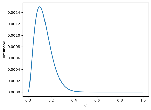
Fig. 13.1 Likelihood function for the default probability#
The likelihood is maximized at a value of θ somewhere around 0.1.
We can locate the maximizer more precisely by finding the grid point with the largest likelihood.
θ_grid[np.argmax(L_values)]
np.float64(0.101)
13.2.4. Maximizing the likelihood with calculus#
Let’s now find the maximizer exactly, using calculus.
We could differentiate \(L\) directly, but differentiating a product of \(n\) terms is awkward.
It is easier to work with the logarithm of the likelihood, called the log likelihood:
Since the logarithm is strictly increasing, \(L\) and \(\ell\) have the same maximizer.
So we can maximize \(\ell\) instead of \(L\).
The advantage is that the logarithm turns products into sums.
Using \(\ln (ab) = \ln a + \ln b\) and \(\ln (a^b) = b \ln a\), we get
Let \(k := \sum_{i=1}^n y_i\) be the number of defaults.
Then \(\sum_{i=1}^n (1 - y_i) = n - k\) is the number of loans repaid, and collecting terms gives
Its derivative is
Assuming that \(0 < k < n\), we set the derivative to zero and multiply through by \(\theta (1 - \theta)\), which gives
This point is a maximum, since the second derivative
is negative everywhere on \((0, 1)\).
Hence the maximum likelihood estimate is
This is the sample mean of the data, or, in other words, the fraction of loans that defaulted.
Let’s check that it agrees with the figure.
k = y.sum()
k / n
np.float64(0.1)
This matches the grid search above, up to the spacing of the grid.
Notice that the estimate is not equal to the true value 0.15.
With only 20 loans, the fraction that defaulted is a noisy guide to θ.
We will see below that the estimate improves as we observe more loans.
13.2.5. Likelihood is not probability#
It is important to be clear about what \(L\) is.
For a fixed θ, the expression in (13.1) is a probability, and summing it over all possible data sets gives one.
As a function of θ with the data fixed, it is not a probability density over θ and need not integrate to one.
That is why we give it a different name.
13.2.6. More data#
Let’s see what happens to the likelihood as we observe more loans.
Exponentiating our expression for \(\ell\) shows that \(L(\theta) = \theta^k (1 - \theta)^{n - k}\), which is quicker to compute than the product when \(n\) is large.
def bernoulli_likelihood(θ, k, n):
    return θ**k * (1 - θ)**(n - k)
Since the likelihood gets very small when \(n\) is large, we divide each curve by its maximum value, so that all the curves peak at one.
(We return to the problem of very small likelihoods below.)
fig, ax = plt.subplots()
for n in (10, 100, 1000):
    y = (rng.random(n) < θ_true).astype(int)
    k = y.sum()
    L = bernoulli_likelihood(θ_grid, k, n)
    ax.plot(θ_grid, L / L.max(), lw=2, label=f'$n = {n}$')
ax.axvline(θ_true, color='k', ls=':', lw=1, label=r'true $\theta$')
ax.set_xlim(0, 0.5)
ax.set_xlabel(r'$\theta$')
ax.set_ylabel('likelihood (normalized)')
ax.legend()
plt.show()
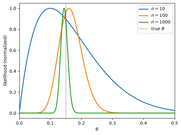
Fig. 13.2 Likelihood functions for increasing sample sizes#
As \(n\) grows, the likelihood concentrates around the true value.
With more data, fewer values of θ are consistent with what we observe.
This is a first sign of the consistency of maximum likelihood, which we study below.
13.3. More examples#
In this section we derive maximum likelihood estimates for three more distributions.
In each case the data \(x_1, \ldots, x_n\) are assumed to be IID draws from a distribution with density or probability mass function \(f(x; \theta)\).
The log likelihood is then
13.3.1. Poisson#
In Fitting Distributions to Data we modeled the number of goals scored in a football match with a Poisson distribution.
The Poisson distribution with parameter λ has probability mass function \(f(x; \lambda) = e^{-\lambda} \lambda^x / x!\), so
Setting the derivative to zero gives
Let’s check this on the goals data.
url = ('https://github.com/QuantEcon/data-lectures/raw/main/'
       'lectures/epl_match_goals.csv')
matches = pd.read_csv(url)
goals = matches['home_goals'] + matches['away_goals']
We compute the log likelihood on a grid of values for λ, using the log probability mass function provided by SciPy.
λ_grid = np.linspace(2, 3.5, 200)
ℓ = [scipy.stats.poisson.logpmf(goals, λ).sum() for λ in λ_grid]

fig, ax = plt.subplots()
ax.plot(λ_grid, ℓ, lw=2)
ax.axvline(goals.mean(), color='k', ls='--', lw=1, label='sample mean')
ax.set_xlabel(r'$\lambda$')
ax.set_ylabel('log likelihood')
ax.legend()
plt.show()
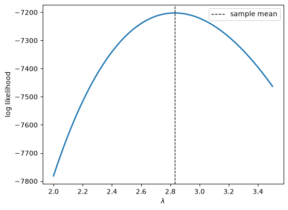
Fig. 13.3 Log likelihood for the Poisson parameter#
The maximum is at the sample mean, as the formula predicts.
λ_grid[np.argmax(ℓ)], goals.mean()
(np.float64(2.829145728643216), np.float64(2.83))
(The two numbers differ slightly only because the grid is finite.)
13.3.2. Normal#
The normal distribution has two parameters, μ and σ, and density
The log likelihood is
Setting the partial derivatives with respect to μ and σ to zero gives
In other words, \(\hat \mu\) is the sample mean of the data, and \(\hat \sigma\) is the sample standard deviation.
(Here the sample standard deviation is computed with divisor \(n\), a point we return to below.)
Let’s look at the log likelihood for the heights of US adult women, which we fitted with a normal distribution in Fitting Distributions to Data.
url = ('https://github.com/QuantEcon/data-lectures/raw/main/'
       'lectures/us_adult_heights.csv')
heights = pd.read_csv(url)
female = heights[heights['sex'] == 'female']['height_cm'].to_numpy()
With two parameters, the log likelihood is a surface, which we display with a contour plot.
We compute \(\hat \mu\) and \(\hat \sigma\) using NumPy’s mean and std
methods, which implement the formulas above, and mark the point
\((\hat \mu, \hat \sigma)\) on the plot.
μ_hat, σ_hat = female.mean(), female.std()

μ_grid = np.linspace(μ_hat - 1.5, μ_hat + 1.5, 200)
σ_grid = np.linspace(σ_hat - 1.2, σ_hat + 1.2, 200)
M, S = np.meshgrid(μ_grid, σ_grid)

def normal_log_likelihood(μ, σ, x):
    n = len(x)
    return (- n / 2 * np.log(2 * np.pi) - n * np.log(σ)
            - ((x - μ)**2).sum() / (2 * σ**2))

Z = np.vectorize(lambda μ, σ: normal_log_likelihood(μ, σ, female))(M, S)

fig, ax = plt.subplots()
cs = ax.contour(M, S, Z, levels=20, cmap='viridis')
ax.plot(μ_hat, σ_hat, 'ko', label='maximum')
ax.set_xlabel(r'$\mu$')
ax.set_ylabel(r'$\sigma$')
ax.legend()
plt.show()
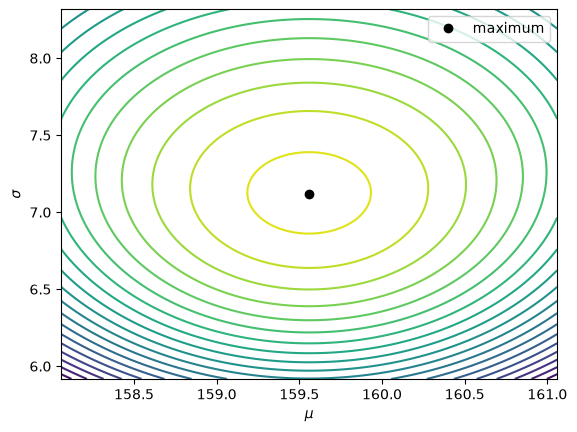
Fig. 13.4 Log likelihood for the normal distribution#
As expected, the log likelihood is maximized at \((\hat \mu, \hat \sigma)\).
Here are the values.
μ_hat, σ_hat
(np.float64(159.5593947270702), np.float64(7.117294168207015))
Notice that \(\hat \sigma\) divides by \(n\) rather than \(n - 1\).
This is also what NumPy computes by default: female.std() uses \(n\), while
female.std(ddof=1) uses \(n - 1\).
For large samples the difference is negligible, but for small samples it is not, as you are asked to check in an exercise.
The normal log likelihood also sheds light on Simple Linear Regression Model.
Suppose that \(y_i = \alpha + \beta x_i + \epsilon_i\), where the errors \(\epsilon_i\) are IID and normal with mean zero and standard deviation σ.
Then, replacing \(x_i - \mu\) by \(y_i - \alpha - \beta x_i\) in (13.2), the log likelihood is
For any σ, maximizing this over α and β is the same as minimizing the sum of squared residuals.
So, with normal errors, ordinary least squares is maximum likelihood.
13.3.3. Pareto#
Our last example is the Pareto distribution from Heavy-Tailed Distributions.
We assume that the minimum value \(\bar x\) is known, so that the only unknown parameter is the tail index α.
The density is \(f(x; \alpha) = \alpha \bar x^\alpha / x^{\alpha + 1}\) for \(x \geq \bar x\), so
Setting the derivative to zero gives
Here’s a function that computes it.
def pareto_mle(x, x_bar=1.0):
    return len(x) / np.sum(np.log(x / x_bar))
For the Bernoulli, Poisson and normal distributions, the maximum likelihood estimates coincide with the method of moments estimates from Fitting Distributions to Data, since both are built from the sample mean and variance.
For the Pareto distribution this is not the case.
We will see below that the difference matters.
13.4. Consistency#
An estimator is called consistent if it converges to the true parameter value as the sample size grows.
Let’s check this by simulation for the Pareto estimate (13.3).
We set \(\bar x = 1\) and α = 1.5, and draw many samples of size \(n\).
To draw from the Pareto distribution we use the inverse transform method: if \(U\) is uniform on \((0, 1)\), then \(\bar x U^{-1/\alpha}\) is Pareto with minimum \(\bar x\) and tail index α.
def pareto_draws(α, size, rng, x_bar=1.0):
    return x_bar * rng.random(size)**(-1 / α)
For each sample size, we compute the estimate on 2,000 independent samples and plot a kernel density estimate (see Observed Distributions) of the results.
α_true = 1.5
num_reps = 2_000
sample_sizes = (50, 200, 1_000, 5_000)

α_grid = np.linspace(0.9, 2.3, 400)
fig, ax = plt.subplots()
for n in sample_sizes:
    x = pareto_draws(α_true, (num_reps, n), rng)
    α_hats = n / np.sum(np.log(x), axis=1)
    kde = scipy.stats.gaussian_kde(α_hats)
    ax.plot(α_grid, kde(α_grid), lw=2, label=f'$n = {n}$')
ax.axvline(α_true, color='k', ls=':', lw=1, label=r'true $\alpha$')
ax.set_xlabel(r'estimate of $\alpha$')
ax.set_ylabel('density')
ax.legend()
plt.show()
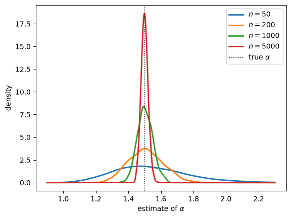
Fig. 13.5 Maximum likelihood estimates of the tail index#
As \(n\) grows, the estimates concentrate on the true value.
This property holds for maximum likelihood estimates in general, under conditions that are satisfied in most applications.
(Proofs can be found in any graduate text on statistics.)
13.5. Maximum likelihood and the method of moments#
In Fitting Distributions to Data we fitted distributions using the method of moments, which chooses parameters so that the moments of the fitted distribution (its mean, variance and so on) match the corresponding moments of the data.
Let’s compare this method with maximum likelihood for the Pareto distribution.
The Pareto distribution has one unknown parameter α, so the method of moments uses one moment, the mean.
This immediately raises a problem.
As we saw in Heavy-Tailed Distributions, the mean of the Pareto distribution is finite only when α > 1.
When α ≤ 1 the mean is infinite, so there is no population mean for the sample mean to match, and the method of moments cannot be used.
When α > 1, the mean is \(\alpha \bar x / (\alpha - 1)\).
Setting this equal to the sample mean \(m_n = \frac{1}{n} \sum_i x_i\) and solving for α gives the method of moments estimate
def pareto_mom(x, x_bar=1.0):
    m = np.mean(x, axis=-1)
    return m / (m - x_bar)
In practice, of course, we do not know α in advance, so we do not know whether the method is valid.
The danger is that the formula can be computed for any sample, since every sample has a finite mean.
Moreover, since every observation is at least \(\bar x\), we have \(m_n > \bar x\), so the formula always returns a value greater than one.
So if the true α is at or below one, the method of moments quietly gives an answer that is on the wrong side of one, suggesting that the mean is finite when in fact it is not.
Even when α > 1, so that the method is valid, heavy tails cause trouble.
When α ≤ 2 the variance is infinite, and, as we saw in Heavy-Tailed Distributions, the sample mean then settles down only slowly, because it is dominated by a few very large draws.
The method of moments estimate inherits this instability.
Maximum likelihood has neither problem.
It works with the density, which is well defined for every α > 0.
Also, the estimate (13.3) depends on the data only through the average of \(\ln (x_i / \bar x)\), and taking logs tames the very large draws.
(In fact, if \(X\) is Pareto, then \(\ln (X / \bar x)\) is exponentially distributed, which is a light-tailed distribution.)
Let’s compare the two estimators by simulation, with samples of size 1,000.
We take α = 0.8, where the method of moments is not valid, and α = 1.5, where it is valid but the variance is infinite.
n = 1_000
fig, axes = plt.subplots(1, 2, figsize=(10, 4))
for ax, α, lims in zip(axes, (0.8, 1.5), ((0.65, 1.2), (1.0, 2.0))):
    x = pareto_draws(α, (num_reps, n), rng)
    α_mle = n / np.sum(np.log(x), axis=1)
    α_mom = pareto_mom(x)
    bins = np.linspace(*lims, 80)
    ax.hist(α_mle, bins=bins, density=True, alpha=0.5,
            label='maximum likelihood')
    ax.hist(α_mom, bins=bins, density=True, alpha=0.5,
            label='method of moments')
    ax.axvline(α, color='k', ls=':', lw=2, label=r'true $\alpha$')
    ax.set_title(rf'$\alpha = {α}$')
    ax.set_xlabel(r'estimate of $\alpha$')
    ax.set_ylabel('density')
    ax.legend()
plt.tight_layout()
plt.show()
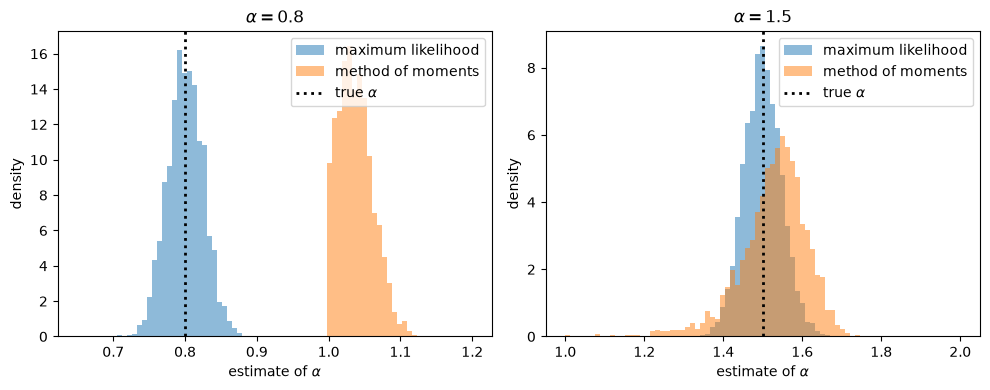
Fig. 13.6 Maximum likelihood and method of moments estimates#
When α = 0.8 (left), the method of moments estimates all lie above one, as predicted, far from the truth, while the maximum likelihood estimates are centered on it.
When α = 1.5 (right), both estimators are concentrated near the truth, but the method of moments estimates are much more dispersed, with a long left tail caused by samples whose mean is inflated by a few very large draws.
Here are the standard deviations of the two sets of estimates for α = 1.5.
np.std(α_mle), np.std(α_mom)
(np.float64(0.047499910499149554), np.float64(0.08460508553363388))
Heavy tails are common in economic data, as we saw in Heavy-Tailed Distributions, and this is one reason why maximum likelihood is the standard method for fitting heavy-tailed distributions.
13.6. Numerical maximum likelihood#
In all the examples so far, we could find the maximizer with pencil and paper.
For many distributions this is not possible, and we have to maximize the log likelihood numerically.
Let’s see how this works for the gamma distribution, which we fitted to house prices by the method of moments in Fitting Distributions to Data.
url = ('https://github.com/QuantEcon/data-lectures/raw/main/'
       'lectures/ames_house_prices.csv')
houses = pd.read_csv(url)
price = houses['price'].to_numpy() / 1_000    # price in thousands of dollars
The gamma distribution has a shape parameter \(a\) and a scale parameter \(s\), both positive.
There is no closed-form expression for the maximum likelihood estimate of \(a\), so we will compute it numerically.
Most numerical optimization routines minimize rather than maximize, so we minimize the negative of the log likelihood.
Why the log likelihood, rather than the likelihood itself?
When we maximized by hand, logs made the calculus easier.
For numerical work there is a second, more important reason.
The likelihood is a product of \(n\) densities, one for each observation, and with thousands of observations this product is too small to represent on a computer.
Here is the likelihood of the house price data at a typical parameter value, \(a = 6\) and \(s = 30\).
u = scipy.stats.gamma(6, scale=30)
np.prod(u.pdf(price))
np.float64(0.0)
The true value is positive, but it is smaller than the smallest positive floating point number, so the computer rounds it to zero.
The log likelihood, which is a sum rather than a product, has no such problem.
np.sum(u.logpdf(price))
np.float64(-16569.572836256266)
For this reason, numerical routines for maximum likelihood always work with the log likelihood.
To keep both parameters positive, we optimize over their logarithms, which can take any real value.
def gamma_neg_log_likelihood(params, x):
    a, s = np.exp(params)
    return -np.sum(scipy.stats.gamma.logpdf(x, a, scale=s))
We need an initial guess, and the method of moments estimates from Fitting Distributions to Data are a natural choice.
m, v = price.mean(), price.var()
a_mom, s_mom = m**2 / v, v / m

result = minimize(gamma_neg_log_likelihood,
                  x0=np.log([a_mom, s_mom]),
                  args=(price,))
a_mle, s_mle = np.exp(result.x)
a_mle, s_mle
(np.float64(6.103147471972235), np.float64(29.623413010946226))
SciPy’s distributions have a fit method that does the same computation, which
we can use as a check.
(Setting floc=0 tells fit not to add a location parameter.)
a_fit, _, s_fit = scipy.stats.gamma.fit(price, floc=0)
a_fit, s_fit
(6.1031472683674854, np.float64(29.623414300572833))
The answers agree.
Here are the two fitted densities.
u_mom = scipy.stats.gamma(a_mom, scale=s_mom)
u_mle = scipy.stats.gamma(a_mle, scale=s_mle)

x_grid = np.linspace(0, price.max(), 400)
fig, ax = plt.subplots()
ax.hist(price, bins=50, density=True, alpha=0.25)
ax.plot(x_grid, u_mom.pdf(x_grid), lw=2, label='method of moments')
ax.plot(x_grid, u_mle.pdf(x_grid), lw=2, label='maximum likelihood')
ax.set_xlabel('sale price (thousands of US$)')
ax.set_ylabel('density')
ax.legend()
plt.show()
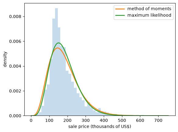
Fig. 13.7 Gamma densities fitted to house prices#
To compare the fits we use the Kolmogorov-Smirnov statistic from Fitting Distributions to Data, the largest vertical gap between the ECDF of the data and the fitted CDF.
def ks_statistic(sample, u):
    "Largest vertical distance between the ECDF of the sample and the CDF of u."
    x_sorted = np.sort(sample)
    n = len(x_sorted)
    F = u.cdf(x_sorted)
    above = np.arange(1, n+1) / n - F     # gap just after each jump
    below = F - np.arange(0, n) / n       # gap just before each jump
    return max(above.max(), below.max())

ks_statistic(price, u_mom), ks_statistic(price, u_mle)
(np.float64(0.07040513845188644), np.float64(0.06727163174892048))
Maximum likelihood gives a slightly closer fit.
Here the two methods give similar answers, because the house price data do not have especially heavy tails.
Remember, though, that maximum likelihood finds the best member of the family we chose, not the best family.
In Fitting Distributions to Data the lognormal family fitted these data better than the gamma family, and no choice of gamma parameters can change that.
Choosing the family is a separate step, for which the Q-Q plots and KS statistics of Fitting Distributions to Data remain the right tools.
13.7. Heavy-tailed returns#
In Fitting Distributions to Data we fitted a Student’s t distribution to monthly returns on Amazon shares, using the method of moments.
We noted there that the fitted degrees of freedom ν were unreliable, because they came from the sample kurtosis, a fourth moment.
Let’s fit the same family by maximum likelihood instead.
data = yf.download('AMZN', '2000-1-1', '2024-1-1', interval='1mo')
prices = data['Close']['AMZN']
returns = prices.pct_change().dropna() * 100
As for the gamma distribution, there is no closed-form expression for the
estimates, so we use the fit method, which maximizes the log likelihood
numerically.
ν_mle, loc_mle, scale_mle = scipy.stats.t.fit(returns)
u_t_mle = scipy.stats.t(df=ν_mle, loc=loc_mle, scale=scale_mle)
ν_mle
np.float64(3.6083739236323873)
For comparison, here is the method of moments fit from Fitting Distributions to Data.
def fit_t_mom(sample):
    m, s = sample.mean(), sample.std()
    ν = 4 + 6 / scipy.stats.kurtosis(sample)
    return scipy.stats.t(df=ν, loc=m, scale=s * np.sqrt((ν - 2) / ν))

u_t_mom = fit_t_mom(returns)
u_t_mom.kwds['df']
np.float64(5.804215121689082)
Maximum likelihood gives a noticeably smaller ν, and hence heavier tails.
It also gives a closer fit.
ks_statistic(returns, u_t_mom), ks_statistic(returns, u_t_mle)
(np.float64(0.04114771740390599), np.float64(0.021858014087628996))
The Q-Q plot from Fitting Distributions to Data confirms that the maximum likelihood fit tracks the extreme returns well.
def qq_plot(sample, u, ax):
    "Plot sample quantiles against the quantiles of the distribution u."
    x_sorted = np.sort(sample)
    n = len(x_sorted)
    p = (np.arange(1, n+1) - 0.5) / n
    ax.plot(u.ppf(p), x_sorted, '.', ms=3, alpha=0.6)
    lo, hi = u.ppf(p[0]), u.ppf(p[-1])
    ax.plot([lo, hi], [lo, hi], 'k--', lw=2)
    ax.set_xlabel('fitted quantiles')
    ax.set_ylabel('sample quantiles')
fig, ax = plt.subplots()
qq_plot(returns, u_t_mle, ax)
plt.show()
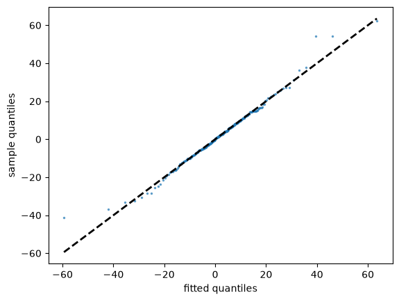
Fig. 13.8 Amazon returns against a t fitted by MLE#
The lesson is the same as for the Pareto simulations: when tails are heavy, sample moments are dominated by a few extreme observations, and maximum likelihood makes better use of the data.
13.8. Exercises#
Exercise 13.1
The exponential distribution with rate λ > 0 has density \(f(x; \lambda) = \lambda e^{-\lambda x}\) for \(x \geq 0\).
Derive the maximum likelihood estimate of λ from IID observations \(x_1, \ldots, x_n\).
Draw a sample of size 500 from the exponential distribution with λ = 2 and check that your formula agrees with
scipy.stats.expon.fit(x, floc=0). (SciPy parameterizes the exponential distribution by the scale \(1/\lambda\).)
Solution
The log likelihood is
Setting the derivative to zero gives \(n / \lambda - \sum_i x_i = 0\), so
Here is the numerical check.
rng = np.random.default_rng(1)
x = rng.exponential(scale=1/2, size=500)

_, scale_fit = scipy.stats.expon.fit(x, floc=0)
1 / x.mean(), 1 / scale_fit
(np.float64(2.05526646936729), 2.05526646936729)
Exercise 13.2
Repeat the consistency simulation of Consistency for the Poisson distribution with λ = 2.7, using sample sizes 10, 100 and 1,000.
Plot histograms of the estimates \(\hat \lambda\) for each sample size.
Solution
rng = np.random.default_rng(2)
λ_true = 2.7
num_reps = 2_000

fig, ax = plt.subplots()
for n in (10, 100, 1_000):
    x = rng.poisson(λ_true, size=(num_reps, n))
    λ_hats = x.mean(axis=1)
    ax.hist(λ_hats, bins=40, density=True, histtype='step', lw=2,
            label=f'$n = {n}$')
ax.axvline(λ_true, color='k', ls=':', lw=1)
ax.set_xlabel(r'estimate of $\lambda$')
ax.set_ylabel('density')
ax.legend()
plt.show()
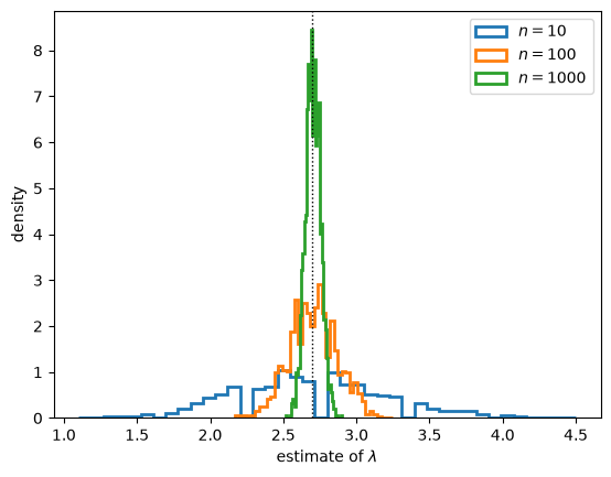
The estimates concentrate on the true value as \(n\) grows.
Exercise 13.3
Suppose that \(x_1, \ldots, x_n\) are IID draws from the uniform distribution on \([0, \theta]\), where θ > 0 is unknown.
Show that the likelihood is \(\theta^{-n}\) when \(\theta \geq \max_i x_i\) and zero otherwise.
Conclude that the maximum likelihood estimate is \(\hat \theta = \max_i x_i\).
Plot the likelihood for a sample of size 10 with θ = 1.
Notice that the maximizer is not found by setting a derivative to zero.
Solution
The density of each observation is \(1/\theta\) on \([0, \theta]\) and zero elsewhere.
If any observation exceeds θ, that observation has zero density, so the likelihood is zero.
Otherwise the likelihood is \((1/\theta)^n = \theta^{-n}\).
Since \(\theta^{-n}\) is decreasing in θ, the likelihood is maximized by the smallest θ that is compatible with the data, which is \(\max_i x_i\).
rng = np.random.default_rng(3)
x = rng.uniform(0, 1, size=10)

θ_grid = np.linspace(0.5, 1.5, 500)
L = np.where(θ_grid >= x.max(), θ_grid**(-len(x)), 0.0)

fig, ax = plt.subplots()
ax.plot(θ_grid, L, lw=2)
ax.axvline(x.max(), color='k', ls='--', lw=1, label=r'$\max_i x_i$')
ax.set_xlabel(r'$\theta$')
ax.set_ylabel('likelihood')
ax.legend()
plt.show()
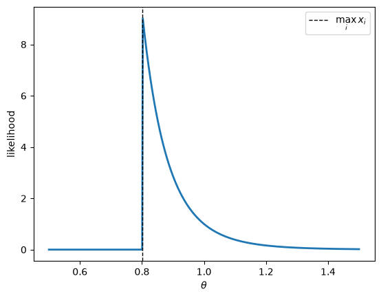
The likelihood jumps up at \(\max_i x_i\) and declines afterwards, so the maximum is at the jump.
Exercise 13.4
The maximum likelihood estimate of \(\sigma^2\) for the normal distribution is \(\hat \sigma^2 = \frac{1}{n} \sum_i (x_i - \bar x)^2\).
Using simulation with samples of size \(n = 5\) from the standard normal distribution, estimate the mean of \(\hat \sigma^2\) and compare it with the true value \(\sigma^2 = 1\).
Repeat the exercise using the divisor \(n - 1\) instead of \(n\).
What do you conclude?
Solution
rng = np.random.default_rng(4)
n, num_reps = 5, 100_000
x = rng.standard_normal((num_reps, n))

x.var(axis=1).mean(), x.var(axis=1, ddof=1).mean()
(np.float64(0.7993801635716414), np.float64(0.9992252044645518))
With divisor \(n\), the mean of the estimates is close to \((n - 1)/n = 0.8\), so the maximum likelihood estimate of \(\sigma^2\) is biased downward.
With divisor \(n - 1\), the mean is close to one, so this estimate is unbiased.
The bias of the maximum likelihood estimate vanishes as \(n\) grows, which is consistent with what we saw in Consistency.