47. Measuring Mobility#

In addition to what’s in Anaconda, this lecture will need the following library:

!pip install quantecon

47.1. Overview#

In Income and Wealth Inequality we measured how unequally income and wealth are distributed at a point in time.

Such measures are snapshots.

While they do provide information on how far apart the rich and the poor are, they tell us nothing about whether the same families stay rich and poor.

This is important because two economies can have identical Lorenz curves and identical Gini coefficients while offering their citizens completely different life prospects.

For example, suppose we are comparing economies with identical wealth distributions.

Suppose further that they fall into one of two cases.

Position is fixed at birth and never changes.
Families rise and fall constantly, and today’s poor household has a good chance of being tomorrow’s rich one.

The difference between these two economies is mobility: the rate at which households change position within the distribution.

Mobility matters for policy.

Attitudes to redistribution, taxation, and our sense of how much opportunity an economy offers all depend on it.

In this lecture we study how to measure mobility when the data take the form of a transition matrix over wealth quantiles.

This is a natural application of the Markov chain theory developed in Markov Chains: Basic Concepts and Markov Chains: Irreducibility and Ergodicity, and it gives us a second use for the Perron-Frobenius theorem.

Note

This lecture draws heavily on the first few sections of the paper “Mobility” by Daniel Carroll, Nicholas Hoffman and Eric R. Young [Carroll et al., 2026].

That paper collects the standard mobility measures in one place, applies them to US wealth data, and then asks whether workhorse macroeconomic models can reproduce what it finds.

Let’s start with some imports.

import matplotlib.pyplot as plt
import numpy as np
import pandas as pd
import quantecon as qe

np.set_printoptions(legacy='1.25')   # print scalars as plain numbers

47.2. Mobility matrices#

47.2.1. From quantiles to a stochastic matrix#

Suppose we observe the wealth of a large number of households at two dates, $s$ and $s + t$.

We sort households by wealth at each date and divide them into $N$ equally sized groups, or quantiles.

(When looking at data we often consider the case $N = 5$, in which case these quantiles are quintiles, each containing 20% of households.)

Now we ask, for each household, which quantile it started in and which quantile it ended in.

Averaging over households gives us a matrix $M$ with typical element

\[ m_{ij} = \mathbb P \{ \text{household $h$ is in quantile } j \text{ at } s+t \mid \text{$h$ was in quantile } i \text{ at } s \} \]

Each row of $M$ is a probability mass function, so $M$ is a stochastic matrix in the sense of Markov Chains: Basic Concepts.

We call $M$ a mobility matrix.

Two points deserve emphasis.

First, $M$ describes relative mobility: it records movement of households relative to one another, not growth in wealth as such.

An economy in which everyone’s wealth doubles has no mobility at all by this definition.

Second, the time unit of the chain is the horizon $t$, which might be five years or twenty.

Much depends on that choice, and we return to it when we look at data.

47.2.2. An example#

Here is a mobility matrix estimated from US data over the five years from 1984 to 1989, which we discuss more fully in a later section.

M_ex = [[0.70, 0.23, 0.05, 0.02, 0.00],
        [0.25, 0.45, 0.22, 0.06, 0.02],
        [0.06, 0.24, 0.44, 0.19, 0.06],
        [0.02, 0.06, 0.22, 0.47, 0.23],
        [0.01, 0.01, 0.06, 0.22, 0.70]]

These figures are published rounded to two decimal places, so the rows do not quite sum to one.

We will need them to, so let’s write a helper that rescales each row.

def normalize_rows(M):
    M = np.asarray(M, dtype=float)
    return M / M.sum(axis=1, keepdims=True)

M_ex = normalize_rows(M_ex)

Row 1 says that a household in the poorest quintile in 1984 had a 70% chance of still being there in 1989, a 23% chance of moving up one quintile, and no chance of reaching the top.

The mass concentrates near the diagonal, and the two extreme quintiles are the stickiest.

To make this concrete, let’s simulate the quintile histories of a few households.

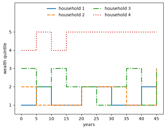
_images/eaa4d6d1340b5a2fe6b27bdfced31347ae53ee4820446c65a81a7e851f0794e9.png — Fig. 47.1 Simulated quintile paths for four households#

Some households wander a long way and others hardly move.

Our task is to summarize this behavior in a single number.

47.2.3. Two benchmarks#

Before choosing a measure, it helps to fix the two extreme cases against which any measure should be calibrated.

Complete immobility is the identity matrix $M = I$.

Every household stays where it starts, forever.

Perfect mobility is the matrix with every entry equal to $1/N$,

\[ M^* = \frac{1}{N} \mathbb 1 \mathbb 1^\top \]

where $\mathbb 1$ is an $N \times 1$ vector of ones.

Here the ending quantile is independent of the starting quantile, so knowing where a household began tells us nothing about where it ends up.

This property is called origin independence, and it is the natural upper reference point for mobility: the distribution is reshuffled completely at every step.

You might object that $M^*$ is not the only matrix with this property.

Indeed, the ending quantile is independent of the starting quantile whenever every row of $M$ is the same, so that $M = \mathbb 1 \psi^\top$ for some probability mass function $\psi$.

Why then single out the uniform case and call it perfect mobility?

The reason is that our quantiles are constructed to hold equal numbers of households at both dates.

The fraction of households ending in quantile $j$ is $\sum_i (1/N) m_{ij}$, and this must equal $1/N$, so

\[ \sum_{i=1}^N m_{ij} = 1 \qquad \text{for every } j \]

In other words, a mobility matrix over equally sized quantiles has columns summing to one as well as rows — it is doubly stochastic.

Now suppose such a matrix also has identical rows, so $M = \mathbb 1 \psi^\top$.

Its $j$-th column sums to $N \psi(j)$, and setting this to one gives $\psi(j) = 1/N$.

So $M^*$ is not one origin-independent matrix among many — within this setting it is the only one.

N = 5
M_immobile = np.identity(N)
M_perfect = np.ones((N, N)) / N

A good measure of mobility should return 0 at $M_{\text{immobile}}$ and 1 at $M_{\text{perfect}}$.

We will see that all four measures below are constructed to do exactly this.

Note

Values above 1 are possible and meaningful.

They arise when a chain reverses ranks systematically — for example a matrix that sends the poorest quintile to the richest with probability one moves households around more than pure chance does.

So 1 marks origin independence, not a maximum.

Such systematic reversal is unusual in ordinary market economies, where wealth is persistent and estimated mobility matrices put most of their mass on or near the diagonal.

All of the empirical matrices we study below score well below 1.

47.3. Four measures of mobility#

Reducing an $N \times N$ matrix to a single number throws away information.

Different measures throw away different information, which is why it is standard practice to report several.

We follow [Carroll et al., 2026] in considering four, each discussed at length in [Dardanoni, 1993].

47.3.1. The Shorrocks index#

The measure of [Shorrocks, 1978] looks only at the diagonal of $M$,

(47.1)#\[\mu_S(M) = \frac{N - \mathrm{trace}(M)}{N - 1}\]

The idea is that $m_{ii}$ is the probability a household in quantile $i$ stays put, so $1 - m_{ii}$ is its probability of escaping.

Rewriting (47.1) as

\[ \mu_S(M) = \frac{N}{N-1} \cdot \frac{1}{N} \sum_{i=1}^N (1 - m_{ii}) \]

shows that $\mu_S$ is the average escape probability, divided by the escape probability $(N-1)/N$ under perfect mobility.

In this sense $\mu_S$ measures the stickiness of initial conditions relative to origin independence.

def shorrocks(M):
    N = len(M)
    return (N - np.trace(M)) / (N - 1)

shorrocks(M_immobile), shorrocks(M_perfect)

(0.0, 1.0)

The measure is completely blind to how probability is arranged off the diagonal.

An economy in which households move from rags to riches in one step and an economy in which the poor become only slightly less poor receive the same score, provided they leave their starting quantile equally often.

47.3.2. Bartholomew’s measure#

The measure of [Bartholomew, 1967] takes the opposite view and looks only at the off-diagonal elements,

(47.2)#\[\mu_B(M) = \frac{1}{N-1} \sum_{i=1}^N \sum_{j=1}^N m_{ij} \, |i - j|\]

The weight $|i-j|$ is the number of quantile boundaries crossed, so transitions that cross several quantiles count for more than transitions to a neighbor.

Up to the factor $1/(N-1)$, this is the expected number of quantiles a household crosses per period.

[Fields and Ok, 1999] describe $\mu_B$ as a measure of total movement.

def bartholomew(M):
    N = len(M)
    i, j = np.indices((N, N))
    return np.sum(M * np.abs(i - j)) / (N - 1)

bartholomew(M_immobile), bartholomew(M_perfect)

(0.0, 2.0)

Notice that $\mu_B$ is not calibrated the same way as $\mu_S$: perfect mobility gives 2 rather than 1.

In fact, a short calculation using $\sum_{i,j} |i-j| = N(N-1)(N+1)/3$ gives

\[ \mu_B(M^*) = \frac{1}{N-1} \cdot \frac{1}{N} \cdot \frac{N(N-1)(N+1)}{3} = \frac{N+1}{3} \]

So to put Bartholomew’s measure on the same footing as the others we rescale,

(47.3)#\[\mu_{NB}(M) = \frac{3}{N+1} \, \mu_B(M)\]

which is the expected number of quantiles crossed, relative to the number crossed under origin independence.

def bartholomew_normalized(M):
    N = len(M)
    return 3 * bartholomew(M) / (N + 1)

bartholomew_normalized(M_immobile), bartholomew_normalized(M_perfect)

(0.0, 1.0)

We report $\mu_B$ when we want the interpretation “quantiles crossed per period” and $\mu_{NB}$ when comparing across measures.

47.3.3. The second eigenvalue#

Our third measure comes from the theory of convergence rather than from counting transitions.

Recall from Markov Chains: Basic Concepts that the distribution $\psi_t = \psi_0 M^t$ converges to the stationary distribution $\psi^*$ when $M$ is everywhere positive.

The Perron-Frobenius theorem tells us that the largest eigenvalue of a stochastic matrix is $\lambda_1 = 1$, and that the rate at which $\psi_t \to \psi^*$ is governed by the modulus of the second largest eigenvalue $\lambda_2$.

A chain that mixes quickly forgets its initial condition quickly, which is exactly what we mean by mobility.

This suggests

(47.4)#\[\mu_{2E}(M) = 1 - |\lambda_2(M)|\]

[Sommers and Conlisk, 1979] show that $\mu_{2E}$ measures the total deviation of $M$ from a matrix of perfect mobility.

def second_eigenvalue(M):
    λ = np.sort(np.abs(np.linalg.eigvals(M)))[::-1]
    return 1 - λ[1]

second_eigenvalue(M_immobile), second_eigenvalue(M_perfect)

(0.0, 1.0)

The identity matrix has $\lambda_2 = 1$ and never mixes, while $M^*$ has $\lambda_2 = 0$ and mixes in a single step.

This measure has a further attraction: for a two-state chain, $|\lambda_2|$ is exactly the autocorrelation of the process, as you are asked to verify in an exercise below.

47.3.4. Mean first passage time#

The final measure asks a question about waiting times: how long does it take a household to reach a given quantile?

Let $T_{ij}$ be the expected number of periods until a household starting in quantile $i$ first arrives in quantile $j$.

To compute it we use first-step analysis: we condition on where the chain goes next, and then use the fact that the problem starting from there looks just like the original one.

Fix the target $j$ and take any starting quantile $i \neq j$.

The household takes one step, which uses up one period no matter where it lands.

That step takes it to quantile $k$ with probability $m_{ik}$, and there are two possibilities.

If $k = j$ the household has arrived, and no further time is needed.

If $k \neq j$ the household must still travel from $k$ to $j$, and the expected time for that remaining journey is $T_{kj}$.

The second case is where the Markov property earns its keep: how long the trip from $k$ takes depends only on $k$, and not on the fact that we reached $k$ by way of $i$.

Averaging over the possible first steps gives

\[ T_{ij} = \underbrace{1}_{\text{the first step}} + \underbrace{m_{ij} \times 0}_{\text{arrived at } j} + \underbrace{\sum_{k \neq j} m_{ik} T_{kj}}_{\text{not yet arrived}} \]

The middle term is zero, so we are left with

(47.5)#\[T_{ij} = 1 + \sum_{k \neq j} m_{ik} T_{kj}\]

Notice that the sum omits $k = j$ not because that case cannot happen, but because it contributes nothing once the household has arrived.

Here is the simplest possible check.

Consider the two-state chain of Markov Chains: Basic Concepts, where an unemployed worker finds a job with probability $\alpha$ each month, and let $i$ be the unemployed state and $j$ the employed one.

The only term in the sum is $k = i$, with $m_{ii} = 1 - \alpha$, so (47.5) reads $T_{ij} = 1 + (1 - \alpha) T_{ij}$, which gives $T_{ij} = 1/\alpha$.

This is exactly right, since the waiting time is geometric with success probability $\alpha$.

Now hold $j$ fixed and read (47.5) as a system of $N-1$ equations in the $N-1$ unknowns $\{T_{ij}\}_{i \neq j}$.

Writing $t$ for the vector of these unknowns and $M_{-j}$ for $M$ with its $j$-th row and $j$-th column deleted, the system is

\[ t = \mathbb 1 + M_{-j} \, t \qquad \text{or} \qquad (I - M_{-j}) \, t = \mathbb 1 \]

which is a linear solve, and is what the code below does for each $j$ in turn.

On the diagonal we use the mean return time to $j$.

By the ergodicity result in Markov Chains: Irreducibility and Ergodicity, an irreducible chain spends a fraction $\psi^*(j)$ of its time in quantile $j$, so visits to $j$ occur on average once every $1/\psi^*(j)$ periods, giving $T_{jj} = 1/\psi^*(j)$.

def mean_first_passage(M):
    """
    Mean first passage matrix T, where T[i, j] is the expected number of
    periods to reach quantile j starting from quantile i.

    The diagonal holds mean return times.

    """
    N = len(M)
    ψ_star = qe.MarkovChain(M).stationary_distributions[0]
    T = np.zeros((N, N))
    for j in range(N):
        idx = [i for i in range(N) if i != j]
        A = np.identity(N - 1) - M[np.ix_(idx, idx)]
        T[idx, j] = np.linalg.solve(A, np.ones(N - 1))
        T[j, j] = 1 / ψ_star[j]
    return T

np.round(mean_first_passage(M_ex), 1)

array([[ 4.4,  5.3,  9.2, 14.4, 22.8],
       [10.1,  4.9,  7.1, 12.3, 20.6],
       [14.3,  7.5,  5.2,  9.4, 17.5],
       [17.3, 10.8,  6.9,  5.5, 12.4],
       [19.2, 13. ,  9. ,  6.1,  5.2]])

Reading the top right entry, a household starting in the poorest quintile waits about 23 periods before first reaching the richest quintile.

Since a period here is five years, that is well over a century.

To get a single number, [Conlisk, 1990] proposes averaging $T$ over a randomly drawn pair of households.

Since quantiles contain equal numbers of households, the relevant weights are $\psi = (1/N, \ldots, 1/N)$, and

\[ \text{MFP}(M) = \psi^\top T \psi \]

is the expected number of periods before one household reaches the quantile of another, both drawn at random.

Under perfect mobility $\text{MFP}(M^*) = N$, so the normalized measure is

(47.6)#\[\mu_{MFP}(M) = \frac{N}{\text{MFP}(M)}\]

which carries units of quantiles per period.

def mfp_measure(M):
    N = len(M)
    ψ = np.ones(N) / N
    return N / (ψ @ mean_first_passage(M) @ ψ)

mfp_measure(M_perfect)

1.0

Unlike the other three, this measure requires irreducibility.

If some quantile cannot be reached from another then the expected waiting time is infinite and $\mu_{MFP} = 0$, regardless of how much movement occurs elsewhere in the matrix.

Note

[Meyer, 1978] gives a closed-form expression for $T$ in terms of a partitioned inverse, which is what [Carroll et al., 2026] use.

The first-step argument in (47.5) is equivalent and easier to remember.

47.3.5. Collecting the measures#

Let’s gather the four measures into one function.

def mobility_measures(M):
    "Return the four mobility measures for stochastic matrix M."
    return pd.Series({'μ_S':   shorrocks(M),
                      'μ_B':   bartholomew(M),
                      'μ_NB':  bartholomew_normalized(M),
                      'μ_2E':  second_eigenvalue(M),
                      'μ_MFP': mfp_measure(M)})

def mobility_table(matrices):
    "Apply the measures to a dict of labelled stochastic matrices."
    return pd.DataFrame({k: mobility_measures(M)
                         for k, M in matrices.items()}).T

The identity matrix is reducible, so we check the perfect mobility benchmark alone.

mobility_table({'perfect mobility': M_perfect}).round(3)

	μ_S	μ_B	μ_NB	μ_2E	μ_MFP
perfect mobility	1.0	2.0	1.0	1.0	1.0

All four measures equal one, apart from the unnormalized $\mu_B$.

47.4. What the measures miss#

Each measure discards information, and the cleanest way to see what is lost is to find matrices that a measure cannot tell apart.

The following examples are adapted from Appendix A.1 of [Carroll et al., 2026], perturbed slightly so that all three chains are irreducible.

Consider three economies with three wealth terciles.

ladder = np.array([[0.50, 0.50, 0.00],
                   [0.25, 0.50, 0.25],
                   [0.00, 0.50, 0.50]])

jumper = np.array([[0.50, 0.10, 0.40],
                   [0.25, 0.50, 0.25],
                   [0.40, 0.10, 0.50]])

sticky = np.array([[0.70, 0.10, 0.20],
                   [0.25, 0.50, 0.25],
                   [0.20, 0.10, 0.70]])

In the ladder economy households can only move to an adjacent tercile, so the poor must pass through the middle class to become rich.

In the jumper economy households leave their tercile just as often, but when they move they usually move all the way.

In the sticky economy households move rarely, but when they do they tend to move a long way.

mobility_table({'ladder': ladder,
                'jumper': jumper,
                'sticky': sticky}).round(3)

	μ_S	μ_B	μ_NB	μ_2E	μ_MFP
ladder	0.75	0.75	0.562	0.5	0.643
jumper	0.75	1.15	0.862	0.6	0.631
sticky	0.55	0.75	0.562	0.5	0.549

Three lessons follow.

The ladder and jumper economies have identical Shorrocks index, because they have the same diagonal.

Shorrocks cannot see that one economy sends households from the bottom to the top in a single step while the other requires two.

The ladder and sticky economies have identical Bartholomew measure, because the extra distance travelled in the sticky economy exactly offsets its lower frequency of movement.

Bartholomew cannot separate frequent small moves from rare large ones.

The second eigenvalue is also equal across the ladder and sticky economies.

Most striking is that the measures disagree about the ranking.

Bartholomew and the second eigenvalue both rank the jumper economy as more mobile than the ladder economy, while mean first passage time ranks it as slightly less mobile.

The reason is that a household in the jumper economy that wants to reach the middle tercile has to wait a long time, since almost all of the movement is between the extremes.

There is, in short, no complete ordering of mobility matrices, and any single index imposes one by fiat.

This is the central message of [Fields and Ok, 1999] and [Dardanoni, 1993], and it is why we report four numbers rather than one.

47.5. Wealth mobility in the US data#

47.5.1. The data#

We now turn to the wealth mobility matrices estimated by [Carroll et al., 2026] from the Panel Study of Income Dynamics (PSID).

The PSID follows the same families over time and includes wealth supplements at irregular intervals between 1984 and 2015.

For each pair of survey years, families are sorted into wealth quintiles in the starting year and in the ending year, and the fraction moving from quintile $i$ to quintile $j$ is recorded.

The authors report matrices at three horizons: short (5–6 years), medium (9–10 years) and long (19–21 years).

We start with three horizons that share the same starting year, 1984.

psid = {}

psid['1984-1989'] = [[0.70, 0.23, 0.05, 0.02, 0.00],
                     [0.25, 0.45, 0.22, 0.06, 0.02],
                     [0.06, 0.24, 0.44, 0.19, 0.06],
                     [0.02, 0.06, 0.22, 0.47, 0.23],
                     [0.01, 0.01, 0.06, 0.22, 0.70]]

psid['1984-1994'] = [[0.63, 0.24, 0.09, 0.03, 0.02],
                     [0.23, 0.41, 0.21, 0.10, 0.05],
                     [0.10, 0.28, 0.33, 0.21, 0.09],
                     [0.05, 0.08, 0.26, 0.37, 0.23],
                     [0.02, 0.03, 0.09, 0.25, 0.61]]

psid['1984-2003'] = [[0.58, 0.25, 0.11, 0.05, 0.02],
                     [0.26, 0.35, 0.22, 0.12, 0.05],
                     [0.09, 0.29, 0.27, 0.22, 0.13],
                     [0.05, 0.11, 0.27, 0.32, 0.26],
                     [0.03, 0.06, 0.11, 0.26, 0.55]]

As before, the published rounding leaves the rows slightly off.

np.array(psid['1984-2003']).sum(axis=1)

array([1.01, 1.  , 1.  , 1.01, 1.01])

psid = {k: normalize_rows(M) for k, M in psid.items()}

We argued above that a mobility matrix over equally sized quantiles should be doubly stochastic.

Let’s see how well the estimated matrices satisfy this.

for label, M in psid.items():
    print(f'{label}:  {M.sum(axis=0).round(3)}')

1984-1989:  [1.041 0.992 0.994 0.962 1.011]
1984-1994:  [1.023 1.036 0.978 0.961 1.001]
1984-2003:  [1.003 1.056 0.975 0.964 1.002]

The columns sum to roughly but not exactly one.

Two things push them off.

The published figures are rounded to two decimal places, and the panel is not perfectly balanced — families leave the sample between the starting and ending years, so the households sorted into quintiles at the two dates are not quite the same set.

We will see the same deviation resurface in the final exercise, where the stationary distribution of these matrices turns out to be close to uniform without being exactly uniform.

Here is what the three matrices look like.

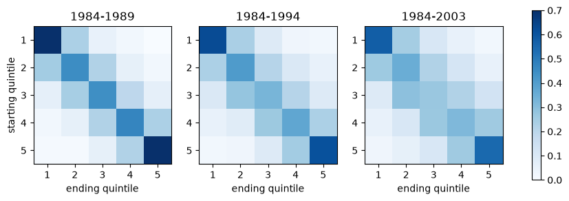
_images/10fc06701b135eef12f380edf2e0170fdca73fbc175574bdb4cd79a658a27c49.png — Fig. 47.2 US wealth mobility matrices at three horizons#

The mass spreads away from the diagonal as the horizon lengthens, which is what we should expect.

There is a good deal of movement even at five years.

Families in the middle three quintiles are more likely to leave their starting quintile than to remain in it, and a household starting in the top quintile has a 30% chance of ending elsewhere.

47.5.2. Mobility rises with the horizon#

Let’s apply our measures.

horizon_table = mobility_table(psid)
horizon_table.round(3)

	μ_S	μ_B	μ_NB	μ_2E	μ_MFP
1984-1989	0.559	0.689	0.345	0.192	0.462
1984-1994	0.664	0.911	0.455	0.306	0.608
1984-2003	0.736	1.044	0.522	0.365	0.683

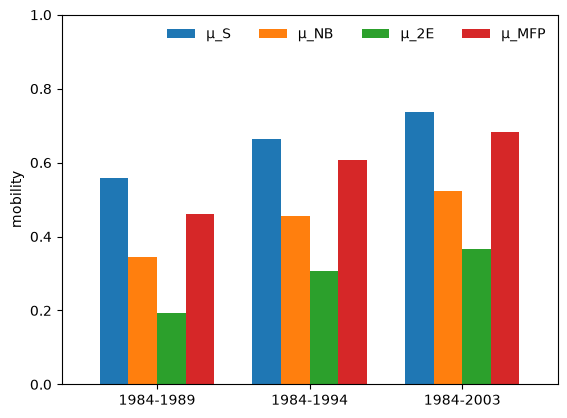
_images/4587d283359e756090a0ab10b26a4a0ec4e05a0c3d65a5fda01db740c798e31d.png — Fig. 47.3 Mobility measures at three horizons#

All four measures agree that mobility rises with the horizon, and they agree by roughly the same proportion.

This is reassuring but not informative: given enough time, any irreducible chain forgets where it started, so every measure must approach one as the horizon lengthens.

The lesson is that mobility measures are only comparable across matrices with the same horizon.

This warning applies with particular force to $\mu_{MFP}$, whose units are quantiles per period — and here a “period” is five years in one column and nineteen in another.

47.5.3. Has mobility declined?#

A more interesting comparison holds the horizon fixed and varies the sample period.

Here are three long-horizon matrices, each spanning about twenty years, starting in 1984, 1989 and 1994.

long_horizon = {}

long_horizon['1984-2003'] = psid['1984-2003']

long_horizon['1989-2009'] = normalize_rows(
                            [[0.56, 0.28, 0.10, 0.04, 0.03],
                             [0.27, 0.37, 0.20, 0.12, 0.05],
                             [0.12, 0.25, 0.29, 0.22, 0.12],
                             [0.08, 0.11, 0.29, 0.32, 0.20],
                             [0.02, 0.05, 0.09, 0.25, 0.60]])

long_horizon['1994-2015'] = normalize_rows(
                            [[0.58, 0.24, 0.11, 0.04, 0.03],
                             [0.28, 0.38, 0.20, 0.10, 0.04],
                             [0.13, 0.25, 0.32, 0.21, 0.08],
                             [0.07, 0.11, 0.24, 0.34, 0.25],
                             [0.03, 0.05, 0.09, 0.25, 0.58]])

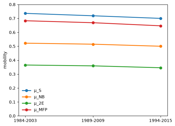
_images/9fab2a41856f5f5a4a486bee660ac27534ac431562c092365c663376633e58c4.png — Fig. 47.4 Long-horizon mobility over three sample periods#

decline_table.round(3)

	μ_S	μ_B	μ_NB	μ_2E	μ_MFP
1984-2003	0.736	1.044	0.522	0.365	0.683
1989-2009	0.719	1.029	0.515	0.359	0.669
1994-2015	0.700	1.000	0.500	0.346	0.647

All four measures fall as we move the twenty-year window forward, suggesting that US wealth mobility has declined since the mid-1980s.

The decline is modest — $\mu_S$ falls from 0.74 to 0.70.

[Carroll et al., 2026] bootstrap the PSID sample to place confidence intervals around these numbers, and conclude that the decline is statistically significant at the medium horizon but not at the long horizon shown here.

47.5.4. Is the quintile chain Markov?#

There is one more question the data let us ask.

So far we have treated each matrix as a separate object.

But if a household’s quintile really were a Markov chain, the twenty-year matrix would be the five-year matrix raised to the fourth power.

Let’s check.

M_short = psid['1984-1989']

comparison = mobility_table(
    {'1984-1994 (data)':  psid['1984-1994'],
     'M^2 (predicted)':   np.linalg.matrix_power(M_short, 2),
     '1984-2003 (data)':  psid['1984-2003'],
     'M^4 (predicted)':   np.linalg.matrix_power(M_short, 4)})

comparison.round(3)

	μ_S	μ_B	μ_NB	μ_2E	μ_MFP
1984-1994 (data)	0.664	0.911	0.455	0.306	0.608
M^2 (predicted)	0.743	1.043	0.522	0.347	0.680
1984-2003 (data)	0.736	1.044	0.522	0.365	0.683
M^4 (predicted)	0.873	1.431	0.716	0.574	0.856

Iterating the five-year matrix predicts substantially more mobility than we observe.

At twenty years the gap is large: $\mu_S$ is 0.87 under the Markov prediction against 0.74 in the data.

Households are therefore more persistent over long horizons than their five-year behavior implies, which means that current quintile alone is not a sufficient statistic for a household’s future position.

Also, unobserved features are at work.

For example, [Carroll et al., 2026] find that a family that makes one large jump through the wealth distribution is significantly more likely to make another, and families holding stocks or private businesses move much more than others.

This matters for modelling.

It means that the state of a realistic model must include something beyond position in the wealth distribution.

47.6. Exercises#

Exercise 47.1

This exercise asks you to check the calibration of the Shorrocks index and explore its range.

Show analytically that $\mu_S(I) = 0$ and $\mu_S(M^*) = 1$, where $M^* = \mathbb 1 \mathbb 1^\top / N$.
Show that $\mu_S(M) \leq N/(N-1)$ for any stochastic matrix $M$, with equality if and only if the diagonal of $M$ is zero.
Hence find a $3 \times 3$ stochastic matrix with $\mu_S(M) > 1$ and confirm your answer in code.
Explain in words what such a matrix does, and why exceeding one is not a defect of the measure.

Solution

For part 1, the identity matrix has $\mathrm{trace}(I) = N$, so $\mu_S(I) = (N - N)/(N-1) = 0$.

The perfect mobility matrix has every diagonal element equal to $1/N$, so $\mathrm{trace}(M^*) = 1$ and $\mu_S(M^*) = (N-1)/(N-1) = 1$.

For part 2, every element of a stochastic matrix is nonnegative, so $\mathrm{trace}(M) \geq 0$, giving $\mu_S(M) \leq N/(N-1)$.

Equality requires $\mathrm{trace}(M) = 0$, which for a nonnegative matrix means every diagonal element is zero.

For part 3, any stochastic matrix with a zero diagonal will do, and the simplest is a cyclic permutation.

M_cycle = np.array([[0.0, 1.0, 0.0],
                    [0.0, 0.0, 1.0],
                    [1.0, 0.0, 0.0]])

shorrocks(M_cycle)

1.5

This is $3/2$, the maximum for $N = 3$.

For part 4, this matrix moves every household out of its current tercile with probability one, which is more movement than origin independence delivers — under $M^*$ a household stays put with probability $1/N$.

So values above one indicate systematic rank reversal rather than an error.

Note that this chain is periodic, so the distribution never converges, even though the chain is irreducible.

Compare the discussion of periodic chains in Markov Chains: Irreducibility and Ergodicity.

Exercise 47.2

Consider the two-state chain from Markov Chains: Basic Concepts,

\[\begin{split} M = \begin{bmatrix} 1 - \alpha & \alpha \\ \beta & 1 - \beta \end{bmatrix} \end{split}\]

with $\alpha, \beta \in (0,1)$ and $\alpha + \beta \leq 1$.

Show that $\mu_S(M) = \mu_{NB}(M) = \mu_{2E}(M) = \alpha + \beta$.
Let $\{X_t\}$ be a stationary chain with this transition matrix, viewed as taking values in $\{0, 1\}$.

Show that its autocorrelation is $\mathrm{corr}(X_t, X_{t+1}) = 1 - \alpha - \beta = |\lambda_2(M)|$.
Verify both results numerically.
Comment on what this tells us about when the choice of mobility measure matters.

Solution

For part 1, the trace is $2 - \alpha - \beta$, so $\mu_S = (2 - (2 - \alpha - \beta))/1 = \alpha + \beta$.

For Bartholomew, only the two off-diagonal terms contribute and each has $|i - j| = 1$, so $\mu_B = \alpha + \beta$, and with $N = 2$ the normalization factor $3/(N+1)$ equals one.

For the eigenvalues, the rows of $M$ sum to one so $\lambda_1 = 1$, and since the eigenvalues sum to the trace we have $\lambda_2 = 1 - \alpha - \beta$, which is nonnegative under our assumption.

Hence $\mu_{2E} = 1 - (1 - \alpha - \beta) = \alpha + \beta$.

For part 2, the stationary distribution is $\psi^* = (\beta, \alpha)/(\alpha + \beta)$, so with $p := \psi^*(1) = \alpha/(\alpha+\beta)$ we have $\mathbb E X_t = p$ and $\mathrm{var}(X_t) = p(1-p)$.

Since $X_t$ is a zero-one variable,

\[ \mathbb E [X_t X_{t+1}] = \mathbb P\{X_t = 1, X_{t+1} = 1\} = p (1 - \beta) \]

Therefore

\[ \mathrm{cov}(X_t, X_{t+1}) = p(1-\beta) - p^2 = p (1 - p - \beta) = p(1-p)(1 - \alpha - \beta) \]

where the last step uses $1 - p = \beta/(\alpha+\beta)$, so that $1 - p - \beta = (1-p)(1 - \alpha - \beta)$.

Dividing by $\mathrm{var}(X_t) = p(1-p)$ gives the result.

α, β = 0.2, 0.3
M2 = np.array([[1 - α, α],
               [β, 1 - β]])

print(f'μ_S  = {shorrocks(M2):.4f}')
print(f'μ_NB = {bartholomew_normalized(M2):.4f}')
print(f'μ_2E = {second_eigenvalue(M2):.4f}')
print(f'α+β  = {α + β:.4f}')

μ_S  = 0.5000
μ_NB = 0.5000
μ_2E = 0.5000
α+β  = 0.5000

mc2 = qe.MarkovChain(M2)
X = mc2.simulate(1_000_000, random_state=0)
print(f'sample autocorrelation = {np.corrcoef(X[:-1], X[1:])[0, 1]:.4f}')
print(f'1 - α - β              = {1 - α - β:.4f}')

sample autocorrelation = 0.4995
1 - α - β              = 0.5000

For part 4, with only two states there is a single way to leave a state and a single distance to travel, so the measures cannot disagree.

Mobility measures start to differ only when $N \geq 3$, because only then is there a distinction between moving far and moving often.

Note that $\mu_{MFP}$ is an exception and differs from the others even at $N = 2$.

mfp_measure(M2), 8 * α * β / ((1 + α + β) * (α + β))

(0.64, 0.64)

Exercise 47.3

The Shorrocks index averages escape probabilities, but a closely related and more interpretable quantity is the expected time a household spends in its current quantile before leaving.

Explain why, for a household currently in quantile $i$, the number of periods until it leaves is geometric with success probability $1 - m_{ii}$, so that the mean sojourn time is $1/(1 - m_{ii})$.
Compute the mean sojourn time in each quintile, in years, for the 1984–1989 matrix.
Repeat for the perfect mobility matrix and comment.

Solution

For part 1, by the Markov property, at each period the household leaves quantile $i$ with probability $1 - m_{ii}$, independently of how long it has already been there.

The number of periods until the first departure is therefore geometric, with mean $1/(1 - m_{ii})$.

For part 2, each period of the 1984–1989 matrix is five years.

sojourn = 5 / (1 - np.diag(psid['1984-1989']))

pd.Series(sojourn.round(1), index=[f'quintile {i}' for i in range(1, 6)],
          name='years')

quintile 1    16.7
quintile 2     9.1
quintile 3     9.0
quintile 4     9.4
quintile 5    16.7
Name: years, dtype: float64

Households remain in the bottom and top quintiles for about 17 years on average, roughly twice as long as in the middle three quintiles.

This is the pattern that [Carroll et al., 2026] find standard incomplete-markets models struggle to reproduce.

For part 3, under perfect mobility every diagonal element is $1/N$.

5 / (1 - np.diag(M_perfect))

array([6.25, 6.25, 6.25, 6.25, 6.25])

A household stays for $N/(N-1) = 1.25$ periods — 6.25 years — which is the minimum consistent with independence rather than zero.

Even with no persistence at all, a household has a one in five chance of drawing its own quintile again.

Exercise 47.4

Take the 1984–1989 matrix $M$ and compute all four mobility measures for $M^k$, $k = 1, \ldots, 20$.

Plot the results and explain what you see.

What does this tell us about comparing mobility measures across horizons?

Solution

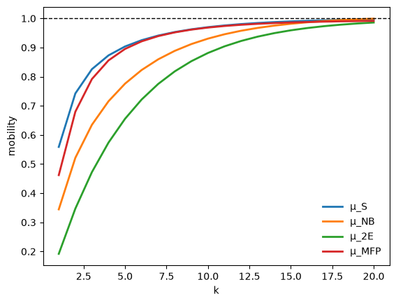
_images/2c9f66a34db8eb8dca311a84ae2de66d3ceb4c52b1ce20e18f537b14431b4e3a.png

Every measure increases monotonically towards one.

This must happen: the matrix is irreducible and aperiodic, so by the Perron-Frobenius theorem the rows of $M^k$ converge to the stationary distribution, and $M^k$ therefore converges to a matrix of the perfect mobility form.

The practical implication is that a mobility measure means nothing without a stated horizon.

Reporting that one economy has $\mu_S = 0.75$ and another $\mu_S = 0.56$ is uninformative if the first figure covers twenty years and the second covers five.

Exercise 47.5

Mobility matrices cannot be completely ordered, and the toy examples above showed one disagreement.

Search for others.

Generate a large number of random $5 \times 5$ stochastic matrices, compute $\mu_{NB}$ and $\mu_{MFP}$ for each, and find a pair that the two measures rank in opposite directions.

Report the pair and explain the disagreement.

Solution

We generate random stochastic matrices by drawing each row from a Dirichlet distribution.

rng = np.random.default_rng(seed=42)

n_draws = 300
draws = [rng.dirichlet(np.ones(5), size=5) for _ in range(n_draws)]
scores = np.array([[bartholomew_normalized(M), mfp_measure(M)] for M in draws])

Some draws are close to reducible, which sends $\mu_{MFP}$ towards zero for reasons that have nothing to do with the comparison we want.

We set those aside.

keep = np.flatnonzero(scores[:, 1] > 0.4)
len(keep)

Now we look for a pair that the two measures rank in opposite directions.

We score each pair by the smaller of the two gaps, so that the winner disagrees substantially on both measures rather than hugely on one.

B, T = scores[keep, 0], scores[keep, 1]
Δ_B = B[:, None] - B[None, :]
Δ_T = T[:, None] - T[None, :]

disagree = np.sign(Δ_B) != np.sign(Δ_T)
score = np.where(disagree, np.minimum(np.abs(Δ_B), np.abs(Δ_T)), 0.0)
a, b = np.unravel_index(np.argmax(score), score.shape)

A, C = draws[keep[a]], draws[keep[b]]
pd.DataFrame({'matrix A': mobility_measures(A),
              'matrix C': mobility_measures(C)}).round(3)

	matrix A	matrix C
μ_S	0.857	0.990
μ_B	1.461	2.264
μ_NB	0.730	1.132
μ_2E	0.634	0.473
μ_MFP	0.840	0.438

Bartholomew ranks matrix C as far more mobile than matrix A, and mean first passage time ranks it as far less mobile.

Here are the two matrices.

np.round(A, 2)

array([[0.43, 0.31, 0.02, 0.16, 0.08],
       [0.07, 0.36, 0.34, 0.19, 0.04],
       [0.26, 0.07, 0.35, 0.05, 0.28],
       [0.07, 0.01, 0.22, 0.02, 0.67],
       [0.2 , 0.11, 0.06, 0.22, 0.42]])

np.round(C, 2)

array([[0.31, 0.01, 0.08, 0.56, 0.04],
       [0.12, 0.09, 0.48, 0.07, 0.24],
       [0.52, 0.04, 0.14, 0.16, 0.14],
       [0.74, 0.02, 0.11, 0.09, 0.04],
       [0.14, 0.21, 0.22, 0.02, 0.41]])

The explanation is visible in the second column of matrix C.

C[:, 1]

array([0.00933477, 0.08952768, 0.03583995, 0.02154579, 0.21255087])

Almost no probability enters quantile 2, so a household waits a very long time to reach it, and the mean first passage measure is dragged down accordingly.

Bartholomew’s measure never notices, because it counts only distance travelled, and matrix C moves plenty of mass between the remaining quantiles — including between the extremes.

The two measures reward different things.

Bartholomew’s measure counts distance travelled and so favours a matrix that shifts mass towards the corners.

Mean first passage time asks how long a household waits to reach an arbitrary quantile, and so penalises any matrix that makes some quantile hard to enter, however much movement occurs elsewhere.

Exercise 47.6

Our function mean_first_passage solves a linear system.

An alternative is to estimate first passage times by simulation.

Write a function that estimates $T_{ij}$ by simulating many paths from state $i$ and recording the first time each path hits state $j$.

Use qe.MarkovChain.simulate, which is JIT compiled.
Compare your estimates to the exact values for the 1984–1989 matrix.
As a second check, compute the stationary distribution used on the diagonal of $T$ by hand — by solving $\psi^* (I - M) = 0$ subject to $\psi^* \mathbb 1 = 1$ — and compare against qe.MarkovChain.stationary_distributions.

Solution

For part 1, we simulate long paths from each starting state and record first hitting times.

def mfp_simulated(M, num_paths=2_000, path_length=400, seed=1234):
    N = len(M)
    mc = qe.MarkovChain(M)
    T = np.zeros((N, N))
    for i in range(N):
        hits = np.full((num_paths, N), np.nan)
        for m in range(num_paths):
            X = mc.simulate(path_length, init=i, random_state=seed + m)
            for j in range(N):
                first = np.flatnonzero(X[1:] == j)
                if first.size > 0:
                    hits[m, j] = first[0] + 1
        T[i] = np.nanmean(hits, axis=0)
    return T

Note that we search X[1:], so that the diagonal records the mean return time rather than zero, matching the convention in mean_first_passage.

T_exact = mean_first_passage(M_short)
T_sim = mfp_simulated(M_short)

print('exact:')
print(np.round(T_exact, 2))
print('simulated:')
print(np.round(T_sim, 2))

exact:
[[ 4.39  5.31  9.24 14.36 22.84]
 [10.12  4.9   7.1  12.33 20.56]
 [14.29  7.54  5.15  9.41 17.53]
 [17.31 10.85  6.93  5.5  12.35]
 [19.22 12.98  8.96  6.11  5.2 ]]
simulated:
[[ 4.38  5.35  8.96 14.47 22.8 ]
 [ 9.76  5.03  7.23 12.35 20.8 ]
 [14.37  7.5   5.34  9.73 17.48]
 [17.34 10.94  6.75  5.77 12.54]
 [19.17 13.02  8.66  6.13  5.64]]

The estimates are close, and the remaining differences are Monte Carlo error.

One bias is worth watching for, though.

Paths that never reach $j$ within path_length steps contribute nothing, so if the paths are too short relative to the rarest transition the estimates are biased downwards.

Try rerunning with path_length=30 to see this.

For part 3, the stationary distribution is a left eigenvector of $M$.

We can find it by solving a linear system, replacing one redundant equation with the normalization $\psi^* \mathbb 1 = 1$.

def stationary_by_hand(M):
    N = len(M)
    A = np.identity(N) - M.T
    A[-1, :] = 1.0              # replace last equation with normalisation
    b = np.zeros(N)
    b[-1] = 1.0
    return np.linalg.solve(A, b)

ψ_hand = stationary_by_hand(M_short)
ψ_qe = qe.MarkovChain(M_short).stationary_distributions[0]

print(np.round(ψ_hand, 6))
print(np.round(ψ_qe, 6))
print(f'max abs difference = {np.max(np.abs(ψ_hand - ψ_qe)):.2e}')

[0.227856 0.204151 0.194078 0.181753 0.192162]
[0.227856 0.204151 0.194078 0.181753 0.192162]
max abs difference = 1.11e-16

The two agree to machine precision.

It is worth noticing that the stationary distribution is not exactly uniform, even though quintiles contain equal numbers of households by construction.

The uniform distribution is stationary for $M$ precisely when $M$ is doubly stochastic, since $\psi^* M = \psi^*$ with $\psi^* = \mathbb 1^\top / N$ says exactly that every column of $M$ sums to one.

So this deviation is the same one we saw in the column sums earlier, and it has the same two sources: the published rounding, and attrition from the panel between 1984 and 1989.

47.7. Further reading#

47.7.1. Measurement theory#

The formal study of mobility indices begins with [Prais, 1955], who applied transition matrices to occupational classes in England, and [Bartholomew, 1967].

[Shorrocks, 1978] put the subject on an axiomatic footing.

He asks what properties a mobility index should satisfy — among them that it equal zero only under complete immobility, that it be invariant to relabelling, that it increase when probability mass is shifted off the diagonal, and that it take a common value under origin independence — and shows that natural-looking lists of such axioms turn out to be mutually inconsistent.

The upshot is that indices necessarily trade one desirable property against another, which is exactly the tension we saw in the toy examples above.

[Dardanoni, 1993] develops the alternative response to that impossibility: rather than forcing a complete ranking, ask when one matrix is unambiguously more mobile than another, and accept a partial order.

[Sommers and Conlisk, 1979] treat the eigenvalue measures, [Conlisk, 1990] the mean first passage approach and the role of monotonicity, and [Kemeny and Snell, 1976] remains the standard reference for the underlying Markov chain theory.

[Fields and Ok, 1999] survey the whole literature and are the best place to start.

[Cowell and Flachaire, 2018] give a more recent treatment that works directly with the underlying distributions rather than with a discretized transition matrix.

Note

This section describes the shape of Shorrocks’ impossibility result rather than stating it formally, since the precise axiom list matters.

Readers should consult [Shorrocks, 1978] directly.

47.7.2. Intergenerational mobility#

This lecture has studied intragenerational mobility: the movement of a given family through the distribution over its own lifetime.

A large parallel literature studies intergenerational mobility, meaning the relationship between the economic position of parents and that of their children.

The headline statistic there is the intergenerational elasticity, the coefficient from regressing a child’s log earnings on the parent’s.

Its most famous appearance is the Great Gatsby curve, named by Alan Krueger in 2012, which plots this elasticity against income inequality across countries [Corak, 2013].

The curve slopes upward: more unequal countries tend to have less intergenerational mobility, with Denmark and Norway at one end and the United States and the United Kingdom at the other.

The interpretation is contested — the relationship is a cross-country correlation across a few dozen data points, and causality could run either way — but the pattern has been influential in policy debate.

[Chetty et al., 2014] use US administrative tax records covering tens of millions of families to show that intergenerational mobility varies enormously within the United States, across commuting zones, and relate that variation to segregation, school quality and family structure.

For wealth specifically, [Hurst et al., 1998] and [Jianakoplos and Menchik, 1997] are early studies using the PSID, and [Benhabib et al., 2019] estimate a model of wealth mobility whose transition matrix we met in Markov Chains: Irreducibility and Ergodicity.

47.7.3. Mobility in economic models#

Everything in this lecture describes data.

The natural next question is whether our standard models of household saving can reproduce it.

The answer, developed in the second half of [Carroll et al., 2026], is that they largely cannot.

A standard incomplete-markets model in the tradition of Bewley, Huggett and Aiyagari, calibrated to match the observed level of wealth inequality, generates far too little short-run mobility.

Households in the model remain in the bottom and top quintiles for around 38 and 63 years respectively, against roughly 15 and 17 in the data, and when they move they move only one quintile at a time.

The reason is that saving is a smoothing device: agents accumulate assets precisely in order to blunt the effect of income shocks on consumption, and this dampening slows their passage through the wealth distribution.

The paper shows that adding idiosyncratic risk to the return on wealth, rather than to labour income, is what brings model mobility into line with the data — consistent with its empirical finding that families making large jumps are the ones holding stocks and private businesses.

It then shows that this matters for policy: across model economies calibrated to identical wealth inequality, the capital income tax rate that households prefer varies with the level of mobility.

That is the case for measuring mobility rather than inequality alone.

Readers interested in the model side should turn to that paper.