14. Estimating Wealth Tax Revenue#
14.1. Overview#
In this lecture we discuss an estimation problem that helps to illustrate the value of maximum likelihood methods.
The problem is: how much revenue would a tax on the wealth of the very rich raise?
This question is topical.
For example, in 2019, US Senator Elizabeth Warren proposed an annual tax on household net worth above 50 million dollars, with a higher rate above one billion dollars (see the proposal).
Emmanuel Saez and Gabriel Zucman estimated that the tax would raise about 2.75 trillion dollars over ten years (letter to Warren), and discuss wealth taxation in detail in [Saez and Zucman, 2019].
Other economists argued that these estimates were too high, and much of the disagreement concerned the number and wealth of the very richest households.
In this lecture we estimate the revenue from a wealth tax using US household survey data.
Estimation is challenging because the richest households are under-represented in the data.
To fill the gap we model the upper tail of the wealth distribution with a Pareto distribution, which we fit by maximum likelihood.
We will use the following imports.
import numpy as np
import matplotlib.pyplot as plt
import pandas as pd
14.2. The tax#
We study a modification of the Warren proposal, with the following marginal tax rates on household net worth:
Net worth |
Marginal rate |
|---|---|
up to $10 million |
0% |
$10 million to $50 million |
1% |
$50 million to $1 billion |
2% |
above $1 billion |
6% |
We can represent this schedule as follows.
Let \(h(w)\) be the tax paid by a household with net worth \(w\).
We can write \(h\) as
where
\(x^+ = \max\{x, 0\}\),
the thresholds are \(t_1 = 10\text{M}\), \(t_2 = 50\text{M}\) and \(t_3 = 1000\text{M}\), and
\(r_1 = 0.01\), \(r_2 = 0.01\) and \(r_3 = 0.04\)
Note that each \(r_k\) is the increment in the marginal rate at \(t_k\).
Here’s how we represent the function in Python.
thresholds = np.array([10e6, 50e6, 1e9])
rate_increases = np.array([0.01, 0.01, 0.04])

def h(w, thresholds=thresholds, rate_increases=rate_increases):
    "Tax paid by a household with net worth w."
    return sum(r * np.maximum(w - t, 0)
               for t, r in zip(thresholds, rate_increases))
Total revenue is the sum of \(h(w)\) over all households in the country.
14.3. The survey estimate#
Our data come from the 2022 Survey of Consumer Finances (SCF), run by the Federal Reserve Board.
The data are a few years old but will be sufficient for this exercise.
url = ('https://github.com/QuantEcon/data-lectures/raw/main/'
       'lectures/us_household_net_worth_2022.csv')
scf = pd.read_csv(url)
scf.head()
| yy1 | y1 | wgt | networth | |
|---|---|---|---|---|
| 0 | 1 | 11 | 3027.956120 | 762100.0 |
| 1 | 1 | 12 | 3054.900065 | 854300.0 |
| 2 | 1 | 13 | 3163.637766 | 678200.0 |
| 3 | 1 | 14 | 3166.228463 | 279600.0 |
| 4 | 1 | 15 | 3235.624715 | 602600.0 |
Each row records the net worth networth of a surveyed household and a survey weight wgt.
The weight is the number of US households that the row represents.
(The weights are used to adjust for undersampling and oversampling of different parts of the wealth distribution.)
w = scf['networth'].to_numpy()
λ = scf['wgt'].to_numpy()

λ.sum() / 1e6     # number of US households, in millions
np.float64(131.3063893834636)
One obvious estimate of total revenue is the following weighted sum.
Here \(\lambda_i\) is the weight of row \(i\).
T_survey = np.sum(λ * h(w))
print(f"survey estimate: ${T_survey / 1e9:.0f} billion per year")
survey estimate: $533 billion per year
14.4. The missing rich#
By design, the SCF excludes some very rich Americans because such people would be too easy to identify.
This means that our estimate is too low.
Let’s count the households in the survey above various levels of wealth.
levels = [10e6, 50e6, 100e6, 1e9, 2.7e9]
pd.DataFrame({
    'survey households': [scf.loc[w > c, 'yy1'].nunique() for c in levels],
    'US households represented': [round(λ[w > c].sum()) for c in levels]},
    index=['> $10M', '> $50M', '> $100M', '> $1B', '> $2.7B'])
| survey households | US households represented | |
|---|---|---|
| > $10M | 676 | 2132856 |
| > $50M | 311 | 185003 |
| > $100M | 194 | 64443 |
| > $1B | 21 | 1655 |
| > $2.7B | 0 | 0 |
The survey contains only about twenty households above one billion dollars, and none above 2.7 billion dollars.
2.7 billion dollars is exactly the wealth that was needed to make the 2022 Forbes 400 list.
These individuals were worth a combined 4.0 trillion dollars (Forbes).
forbes_count = 400
forbes_cutoff = 2.7e9
forbes_wealth = 4.0e12

print(f"total wealth in the survey: ${np.sum(λ * w) / 1e12:.0f} trillion")
total wealth in the survey: $139 trillion
So, in 2022, the Forbes 400 held about 3% of US household wealth, and all of this wealth is missing from the survey.
How much tax would the Forbes 400 pay?
We only know their combined wealth, not the wealth of each member, so we cannot simply apply \(h\) to each member.
But every member is worth more than one billion dollars, and above that level the tax is simple: a member with wealth \(w\) pays \(h(1\text{B})\) on their first billion, plus 6% of the rest.
Adding this up over all members gives
which depends only on their combined wealth.
tax_on_first_billion = h(1e9)                # paid in full by every member
wealth_above_billion = forbes_wealth - forbes_count * 1e9
forbes_tax = forbes_count * tax_on_first_billion + 0.06 * wealth_above_billion
print(f"tax owed by the Forbes 400: ${forbes_tax / 1e9:.0f} billion per year")
tax owed by the Forbes 400: $224 billion per year
This is a large amount relative to the survey estimate, and it is entirely missed by \(\hat T_S\).
There is a second, subtler problem.
Even where the survey does contain very rich households, it contains very few of them, so the survey estimate of revenue from the top bracket rests on a handful of observations and is highly uncertain.
14.5. A Pareto model of the upper tail#
To deal with these problems we need a model of the upper tail of the wealth distribution, which we can estimate from the part of the tail the survey observes and then extend to the part it misses.
As discussed in Heavy-Tailed Distributions, the standard model is the Pareto distribution, going back to Vilfredo [1896].
There is strong empirical support for this choice [Saez and Zucman, 2016], [Vermeulen, 2018].
There is also theoretical support: many models in which fortunes grow at random rates generate Pareto upper tails [Gabaix, 2016], [Jones, 2015], [Benhabib and Bisin, 2018].
Recall from Heavy-Tailed Distributions that if wealth \(W\) has a Pareto tail with tail index α above some threshold \(u\), then
Taking logs, \(\ln \mathbb{P}\{W > x\}\) is a linear function of \(\ln x\) with slope \(-\alpha\).
So a Pareto tail shows up as a straight line when we plot the counter CDF (the probability of exceeding \(x\)) against \(x\) on log-log axes.
Let’s plot the counter CDF of the survey data, using the weights so that each row counts in proportion to the households it represents.
def weighted_ccdf(x_grid, w, λ):
    "Fraction of households with wealth above each point of x_grid."
    return np.array([λ[w > x].sum() for x in x_grid]) / λ.sum()
x_grid = np.geomspace(1e6, 2.5e9, 300)

fig, ax = plt.subplots()
ax.loglog(x_grid, weighted_ccdf(x_grid, w, λ), lw=2, label='survey')
ax.axvline(10e6, color='k', ls=':', lw=1)
ax.set_ylim(1e-8, 1)
ax.set_xlabel('net worth (US$)')
ax.set_ylabel('fraction of households above')
ax.legend()
plt.show()
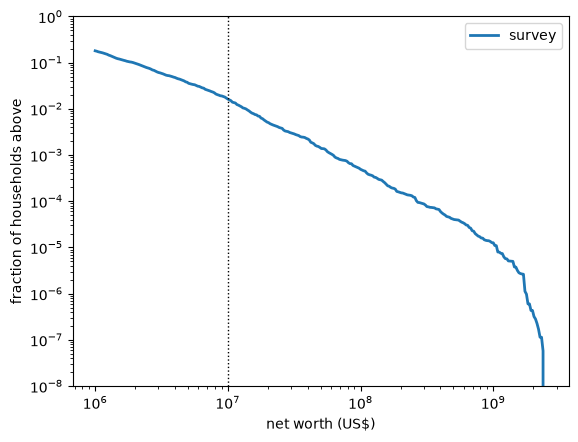
Fig. 14.1 Counter CDF of US household wealth#
Below about 10 million dollars (the dotted line), the curve bends, so the distribution is not Pareto there.
Above 10 million dollars it is close to a straight line.
At the far right the curve plunges, because the survey data stop just below 2.4 billion dollars.
We therefore fit a Pareto tail above the threshold \(u = 10\) million dollars, which is also where our tax begins.
14.6. Estimating the tail index#
In Maximum Likelihood Estimation we found that the maximum likelihood estimate of the tail index, given observations \(x_1, \ldots, x_n\) above a known threshold \(u\), is
Here we have to account for the weights.
If row \(i\) represents \(\lambda_i\) households, then it contributes \(\lambda_i\) copies of its log density to the log likelihood of the population:
Repeating the calculation in Maximum Likelihood Estimation with these weights gives
def tail_index(u, w, λ):
    "Weighted maximum likelihood estimate of the Pareto tail index above u."
    above = w > u
    return λ[above].sum() / np.sum(λ[above] * np.log(w[above] / u))

u = 10e6
α_hat = tail_index(u, w, λ)
α_hat
np.float64(1.5624405884551842)
This is close to published estimates for the United States, which are around 1.5 [Vermeulen, 2018].
14.7. The Pareto estimate of revenue#
With the tail estimated, we can compute revenue from the model instead of from the survey.
Let \(N_u\) be the number of households with wealth above \(u\), which we estimate from the survey weights.
N_u = λ[w > u].sum()
N_u
np.float64(2132856.3510950943)
Revenue is \(N_u\) times the average tax paid by a household above \(u\).
Using (14.1), this average is
For a Pareto tail above \(u\) and a threshold \(t \geq u\), a short calculation shows that
provided that α > 1.
(When α ≤ 1 the integral is infinite, so the expected tax is infinite too.)
Putting these together gives the Pareto estimate of revenue:
def expected_excess(t, α, u):
    "Expected value of (W - t)^+ for a Pareto tail above u, with t >= u."
    return u**α * t**(1 - α) / (α - 1)

def pareto_revenue(α, u, N_u,
                   thresholds=thresholds, rate_increases=rate_increases):
    "Pareto estimate of revenue, for a tail above u containing N_u households."
    return N_u * np.sum(rate_increases * expected_excess(thresholds, α, u))

T_pareto = pareto_revenue(α_hat, u, N_u)
print(f"Pareto estimate: ${T_pareto / 1e9:.0f} billion per year")
Pareto estimate: $646 billion per year
14.8. Comparing the two estimates#
The Pareto estimate is higher than the survey estimate.
To see where the difference comes from, let’s break revenue down by bracket.
The revenue from bracket \(k\) is the tax on wealth between \(t_k\) and \(t_{k+1}\), at the marginal rate for that bracket.
marginal_rates = np.cumsum(rate_increases)
upper = np.append(thresholds[1:], np.inf)

survey_by_bracket = [np.sum(λ * m * np.clip(np.minimum(w, t_up) - t, 0, None))
                     for t, t_up, m in zip(thresholds, upper, marginal_rates)]

def excess_between(t, t_up, α, u):
    "Expected wealth between t and t_up, for a Pareto tail above u."
    top = expected_excess(t_up, α, u) if np.isfinite(t_up) else 0.0
    return expected_excess(t, α, u) - top

pareto_by_bracket = [N_u * m * excess_between(t, t_up, α_hat, u)
                     for t, t_up, m in zip(thresholds, upper, marginal_rates)]

table = pd.DataFrame({'survey': survey_by_bracket,
                      'Pareto': pareto_by_bracket},
                     index=['$10M-$50M at 1%', '$50M-$1B at 2%', 'above $1B at 6%'])
table.loc['total'] = table.sum()
(table / 1e9).round(0)     # billions of dollars per year
| survey | Pareto | |
|---|---|---|
| $10M-$50M at 1% | 227.0 | 226.0 |
| $50M-$1B at 2% | 273.0 | 250.0 |
| above $1B at 6% | 32.0 | 171.0 |
| total | 533.0 | 646.0 |
In the first bracket, where the survey has hundreds of households, the two estimates are almost identical.
This is reassuring, since it tells us that the Pareto model describes the part of the tail that the survey observes well.
The estimates diverge as we move up, and in the top bracket the Pareto estimate is several times larger.
This is exactly where the survey is thin and then stops, and where our concern about missing households applies.
14.9. A check against the Forbes 400#
The Pareto model makes predictions about households that are not in the survey, and we can check them against the Forbes 400.
According to the model, the number of households with wealth above the Forbes cutoff \(c = 2.7\) billion dollars is \(N_u (u / c)^{\alpha}\).
The average wealth of these households is \(\alpha c / (\alpha - 1)\), which follows from (14.2) by setting \(u = t = c\) and adding \(c\).
n_forbes_model = N_u * (u / forbes_cutoff)**α_hat
wealth_forbes_model = n_forbes_model * α_hat * forbes_cutoff / (α_hat - 1)

pd.DataFrame({'Pareto model': [n_forbes_model, wealth_forbes_model / 1e12],
              'Forbes': [forbes_count, forbes_wealth / 1e12]},
             index=['households above $2.7B', 'their wealth ($ trillion)']).round(1)
| Pareto model | Forbes | |
|---|---|---|
| households above $2.7B | 338.9 | 400.0 |
| their wealth ($ trillion) | 2.5 | 4.0 |
The model predicts somewhat fewer households at this level than Forbes finds, and considerably less wealth, but it gets the orders of magnitude right.
This is a demanding test, since the model was estimated entirely from survey households worth less than 2.4 billion dollars.
We can see this graphically, by extending the fitted Pareto line beyond the survey data and adding the Forbes 400 as a single point.
N = λ.sum()
x_fit = np.geomspace(u, 1e11, 100)

fig, ax = plt.subplots()
ax.loglog(x_grid, weighted_ccdf(x_grid, w, λ), lw=2, label='survey')
ax.loglog(x_fit, (N_u / N) * (u / x_fit)**α_hat, 'k--', lw=2,
          label='fitted Pareto tail')
ax.loglog(forbes_cutoff, forbes_count / N, 'o', ms=8, label='Forbes 400')
ax.set_ylim(1e-9, 1)
ax.set_xlabel('net worth (US$)')
ax.set_ylabel('fraction of households above')
ax.legend()
plt.show()
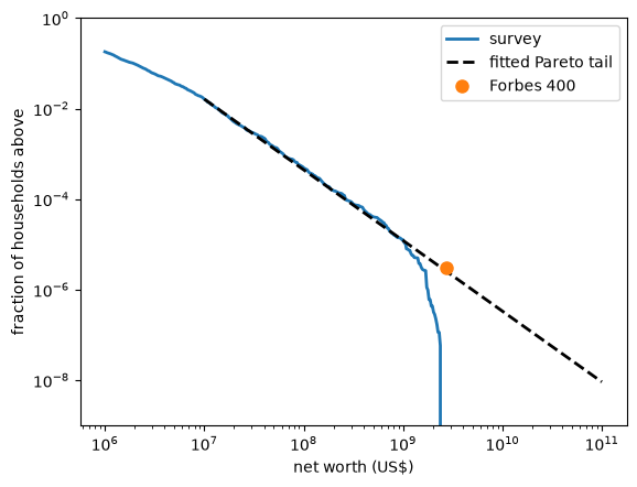
Fig. 14.2 Fitted Pareto tail and the Forbes 400#
The Forbes point lies a little above the fitted line.
There are several possible reasons.
The estimate of α is uncertain, and a slightly smaller value would pass through the Forbes point.
The very top of the distribution may have a heavier tail than the range from which we estimated α.
Rich households may be less likely to respond to the survey, which biases estimates of α upward [Vermeulen, 2018].
Forbes counts individuals and families using its own valuations, which differ from the survey’s definition of a household’s net worth.
The comparison suggests that, if anything, our Pareto estimate of revenue is conservative.
14.10. How much does α matter?#
The formula for \(\hat T_P\) contains the term \(\hat \alpha - 1\) in the denominator.
So, as α falls toward one, estimated revenue rises without bound.
Let’s plot revenue against α.
α_values = np.linspace(1.3, 2.0, 100)
revenue = [pareto_revenue(a, u, N_u) for a in α_values]

fig, ax = plt.subplots()
ax.plot(α_values, np.array(revenue) / 1e9, lw=2, label='Pareto estimate')
ax.axhline(T_survey / 1e9, color='C1', ls='--', lw=2, label='survey estimate')
ax.axvline(α_hat, color='k', ls=':', lw=1)
ax.set_xlabel(r'tail index $\alpha$')
ax.set_ylabel('revenue (US$ billion per year)')
ax.legend()
plt.show()
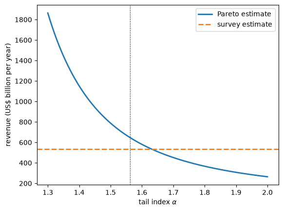
Fig. 14.3 Pareto estimate of revenue against the tail index#
Moving α from 1.6 to 1.4, a change well within the range of sampling uncertainty (see this exercise), roughly doubles estimated revenue.
This sensitivity is one reason why estimates of wealth tax revenue are so contested.
Finally, all of our estimates are mechanical: they assume that households do not change their behavior in response to the tax.
In practice, wealthy households may respond by moving assets, changing how assets are valued, or avoiding the tax in other ways, and the size of these responses is a central question in the policy debate [Saez and Zucman, 2019].
14.11. Exercises#
Exercise 14.1
Warren’s original proposal taxed net worth above 50 million dollars at 2% and net worth above one billion dollars at 3%.
Compute the survey estimate and the Pareto estimate of revenue under this schedule.
Compare them with the Saez and Zucman estimate of about 275 billion dollars per year (2.75 trillion dollars over ten years).
Solution
We pass the new thresholds and rate increases to our functions.
warren = dict(thresholds=np.array([50e6, 1e9]),
              rate_increases=np.array([0.02, 0.01]))

T_s = np.sum(λ * h(w, **warren))
T_p = pareto_revenue(α_hat, u, N_u, **warren)
print(f"survey estimate: ${T_s / 1e9:.0f} billion per year")
print(f"Pareto estimate: ${T_p / 1e9:.0f} billion per year")
survey estimate: $289 billion per year
Pareto estimate: $335 billion per year
Both estimates are of the same magnitude as the Saez and Zucman figure.
Their estimate differs from ours in several ways: it covers the years 2019 to 2028, uses different data for the top of the distribution, and includes an allowance for tax avoidance.
The comparison is therefore only a rough one.
Exercise 14.2
The estimate \(\hat \alpha\) is subject to sampling variation.
One way to measure this is the bootstrap: draw a new sample of households, with replacement, from the survey households, recompute the estimate, and repeat many times.
Since each household appears in five rows, resample households (identified by
yy1) rather than rows.
Use 200 bootstrap samples to compute a 90% interval for \(\hat \alpha\) at \(u = 10\) million dollars, and the corresponding interval for \(\hat T_P\).
Solution
rng = np.random.default_rng(1234)
rows_by_household = scf.groupby('yy1').indices
households = np.array(list(rows_by_household.keys()))

α_boot, T_boot = [], []
for _ in range(200):
    draw = rng.choice(households, size=len(households))
    idx = np.concatenate([rows_by_household[hh] for hh in draw])
    w_b, λ_b = w[idx], λ[idx]
    a = tail_index(u, w_b, λ_b)
    α_boot.append(a)
    T_boot.append(pareto_revenue(a, u, λ_b[w_b > u].sum()))

print("90% interval for α:", np.percentile(α_boot, [5, 95]).round(2))
print("90% interval for revenue ($ billion):",
      (np.percentile(T_boot, [5, 95]) / 1e9).round(0))
90% interval for α: [1.43 1.71]
90% interval for revenue ($ billion): [481. 964.]
The interval for α is roughly ±0.15 around the estimate.
The interval for revenue is wide, reflecting the sensitivity to α discussed above.
Exercise 14.3
The survey estimate and the Pareto estimate agree in the first bracket, where the survey has many observations.
This suggests a hybrid estimate: use the survey for households below 50 million dollars and the Pareto model (still fitted above \(u = 10\) million dollars) for the rest.
Compute it.
Hint: a household with wealth \(W > c = 50\) million dollars pays \(0.01 (c - 10\text{ million})\) on the first bracket, plus \(0.02 (W - c) + 0.04 (W - 1 \text{ billion})^+\).
Solution
Averaging the hint over the Pareto tail and multiplying by the number of households, the revenue from households above \(c\) is
where \(N_c = N_u (u / c)^\alpha\) is the number of households above \(c\).
c = 50e6
below = w <= c
T_below = np.sum(λ[below] * h(w[below]))

N_c = N_u * (u / c)**α_hat
T_above = (N_c * 0.01 * (c - 10e6)
           + N_u * (0.02 * expected_excess(c, α_hat, u)
                    + 0.04 * expected_excess(1e9, α_hat, u)))

print(f"hybrid estimate: ${(T_below + T_above) / 1e9:.0f} billion per year")
hybrid estimate: $643 billion per year
The hybrid estimate lies between the survey and Pareto estimates, and is close to the Pareto estimate, since most of the difference between the two comes from the top brackets.